Detect and fit both halves of a split frame as one emitter, sharing x, y and z: adds the photon ratio that tells the two colours apart.
The detection, the pairing of the two halves' peaks, the ROIs and the global fit are those of Gaussian 2D 2C, which explains them step by step: each half is thresholded on its own, the secondary peaks are mapped onto the main half, peaks within 4 pixels are merged into one candidate and peaks without a partner are kept, and a ROI is cut in each half and both are fitted at once by maximum likelihood. What is new here is the model in each ROI, where it comes from, and z.
Both uses give photons back as photons. Left, two colours: molecules of 2000 photons with a quarter in the secondary half, fitted with the photons free – each half's photons and their sum, against the truth (grey). Right, biplane: molecules that split as the beads did, fitted with one photon number, which is the total.
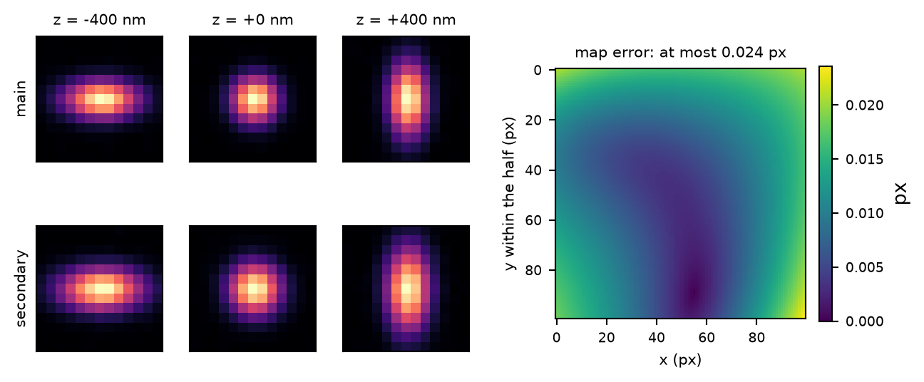
The calibration. Left: the PSF model of each half at three heights, as the fit sees them – the same astigmatism, the secondary half's spot a little wider. Right: how far the calibration's transformation, measured on nine bead pairs, is from the true one over the secondary half, in pixels.
What linking buys. Molecules simulated at known heights from the true PSF (2000 photons split evenly between the halves, 10 background photons per pixel in each) and fitted with the calibration above: the scatter about the truth (dots) and the precision the fit reports (lines), from the main half alone (orange) and from both halves with x, y and z linked (blue). z is about 1.4 times more precise, near the  of two equal looks.
The colour does not depend on the height. Two dyes simulated at known heights, putting 25 % and 75 % of their light into the secondary half, fitted as above: the fitted ratio of each molecule against its true z.
With the photons split evenly and two halves whose PSFs change with z in the same way, each half contributes the same, and the variance of z is half that of one half alone:  shrinks by
  . A dye that puts most of its light into one half gains less, since the other half adds little; and because x, y and z are linked, the photons of both halves count in every one of them.
the plane sum averaged over the focal plane and the two planes either side of it ( the calibration's step). Both PSFs are divided by
  , and
, and  is stored with each, so
  .
.
Clipping keeps a little of the noise, the part above zero – 0.7% of a bright half's signal and 2.7% of a dim one, from 9 beads – which the fit's background mostly takes. Counted as light, it read the photons 1.5% high and the ratio 0.005 high; counted before clipping, the photons come back within 0.7% and the ratio within 0.003, from 9 beads and from 27. Why clip at all, when the fit keeps its model positive anyway? Because the likelihood weighs each pixel by  : a negative dip in the PSF, times a bright molecule's photons, brings the model close to zero wherever the background is low, and a pixel there with a photon in it outweighs the rest. Unclipped, at a photon of background, z scattered by 55 nm where clipped it scatters by
| setting | default | what it does |
|---|
| source – Where the frames come from. |
file
source.path | – | Any file of the acquisition: a Micro-Manager TIFF series, an NDTiff directory, one image out of a folder written one file per frame, or a simulation (*.sim.yaml, File > Simulate). |
first frame (more)
source.start | 0 | Frames before this one are skipped. |
last frame (more)
source.stop | auto | Auto: to the end. at least 1 |
live
source.live | off | The file is still being written: fit what is there and keep watching for new frames. |
stop after (more)
source.live_timeout | 30 s idle | Live: give up after this long without a new frame. at least 1 s idle |
frames per block (more)
source.chunk | 200 | Frames read and detected at once; only memory and speed depend on it. at least 1 |
| camera – ADU -> photons and pixel -> nm. Empty fields come from the file. |
camera
camera.camera | auto | Auto: identified from the file's metadata. |
preset
camera.preset | - | A camera YAML; fills the fields below. |
conversion
camera.conversion | auto | Photoelectrons per count; auto: from the file or the camera database. |
offset
camera.offset | auto | The count of a pixel that saw no light. |
pixel size
camera.pixelsize_um | auto | The pixel's size in the sample, after the magnification. |
pixel size y (more)
camera.pixelsize_y_um | auto | Auto: square pixels, the same as in x. |
EM gain on
camera.em_on | auto | An EMCCD with its electron multiplication on: the counts are divided by the gain, and the noise is doubled. |
EM gain
camera.emgain | auto | The EM gain the camera was set to. |
read noise (more)
camera.read_noise_e | auto | Rms per pixel; auto: 1 without EM gain (an sCMOS), 0 with it. |
| detection – Finding candidates in the filtered image. |
filter
detection.filter | difference of Gaussians | What the frame is smoothed with before maxima are looked for; the difference of Gaussians also removes a smooth background. Choices: difference of Gaussians; Gaussian |
filter sigma
detection.sigma | 1.2 pix | The width of the smoothing: about the PSF's. at least 0.1 pix |
cutoff
detection.cutoff_mode | dynamic (x noise) | Dynamic: set per frame from the noise of the filtered image; absolute: a fixed value. Choices: dynamic (x noise); absolute (photons) |
cutoff value
detection.cutoff | 1.7 | Lower finds dimmer molecules, and more noise. |
| model – A dual-colour calibration, and which parameters the channels share. |
calibration
model.calibration | – | From Bead calibration in Dual colour mode. Made once per microscope configuration: the same objective, dichroic, filters, camera settings and split as the data. It records whether the beads were taken with EM gain, and data taken the other way is warned about (an EM register mirrors the image, and the PSF with it). The first frames are checked against its geometry: a calibration made on another camera ROI is refused, and a movie with no camera ROI in its metadata is taken to start at the chip's corner, with a warning. |
link x, y
model.link_xy | on | One position for both channels, through the registration; unlink only to check the transform. Unlinked, each half fits its own position. The table's position is the main half's, and dx_nm_ch1, dy_nm_ch1 say how far the secondary half put the molecule from where the calibration's transformation expects it: a check of the calibration on this data, whose median should be near 0. Relink for the real fit. |
link z
model.link_z | on | One z for both channels: this is the sqrt(2). Unlinked, each half fits its own z. z_nm is the main half's – the precision of one half – and dz_nm_ch1 is the secondary half's z minus it, which should scatter about 0 at every height if the two PSF models share their focus. |
link photons
model.link_photons | off | Off for two colours – the photon ratio is what tells the dyes apart; on for biplane. On for biplane, off for two colours. Linked, photons is the total and ratio is 0 for every localization – there is no split left to measure, and colour assignment has nothing to work with – but z is more precise still, since both halves' photons count as one. |
link background (more)
model.link_background | off | One background for both halves; off: each half fits its own. |
photon ratio (more)
model.photon_ratio | auto | Secondary / main, used when the photons are linked; auto: the split the calibration's two PSFs carry. Only used with link photons on; with the photons free it has no effect. Leave it empty: the calibration's PSFs already carry the beads' split, which is the molecules' too when the photons can be linked at all (biplane, one dye). Give it only when the molecules split differently from the beads – a narrow-band dye behind a splitter whose transmission depends on colour. |
| fit – Everything about the fit that is not the camera or the PSF model. |
ROI size
fit.roisize | 13 pix | The square cut around each candidate and fitted. Both ROIs have this size. As for Spline 3D it should hold the widest, most defocused spot, and stay inside the calibration's lateral size. at least 5 pix |
iterations (more)
fit.iterations | 50 | The most steps a fit may take. at least 1 |
ROIs per fit (more)
fit.max_block_rois | 15000 | How many are collected before they are fitted together; speed and memory only. at least 100 |
threads (more)
fit.n_threads | 0 | 0: one per core. |
max fit distance (more)
fit.max_fit_distance | auto | Reject fits that ran off; auto: keep all. |
units
fit.output_unit | nm | The unit of the positions in the table. Choices: nm; pixel; pixel+nm |
| output |
save HDF5
output.save | on | Write the table to a file as it is fitted. |
file
output.path | – | Filled from the source: <acquisition>_locs.hdf5 next to the folder the images are in. |
raw frames (more)
output.raw_frames | 50 | Camera frames kept with the table, in photons, after their average; 0: none. 50 is enough to see what the camera saw at the start, the end and a few points between. Each kept frame costs its size in the file: for a 256 x 256 ROI about a quarter of a megabyte, for a full 2048 x 2048 sCMOS chip 16 MB, so fifty of those are 800 MB – set fewer there. |
show image tags
output.show_tags | PIZStage | Image tags drawn when the fit is done, names or parts of names; empty: none (Analysis/Process/Image Tags). PIZStage draws the piezo position, which shows at once whether the focus lock held. On a microscope whose piezo has another name, put that name (or part of it) here. Every tag that changed is kept in the file whatever this says; Analysis/Process/Image Tags draws any of them later.
|
| after the fit – What is run over the finished table, before it is saved. |
assign colours
finish.assign_colors | on | Split the localizations by their photon ratio and write channel (Analysis/Dual-Color/AssignColors). |
drift correction
finish.drift | none | Estimate the drift from the finished table and subtract it from every localization. Off by default: it is minutes of work on a dataset it cannot see beforehand. With z in the table, both RCC and COMET correct z as well unless their correct z says otherwise. Choices: none; RCC; COMET |
| colour assignment |
method
finish.colors.mode | split at the minima | A cut in r, or a posterior per localization. Choices: split at the minima; probabilistic |
colours
finish.colors.colors | 2 | How many species the histogram of r holds. 1 to 6 |
exclusion dr
finish.colors.exclusion | 0.05 | Minima: leave this much of r on either side of a boundary unassigned. |
sigma
finish.colors.tolerance | 3 | Probabilistic: a colour is given only within this many sigma of its expected split, the sigma being that localization's own photon statistics plus any extra spread. 0: assign to the nearest colour however far away. |
keep the tails
finish.colors.keep_tails | off | Probabilistic: apply the sigma test only between the outermost colours, so a localization more extreme than the first or the last mode is kept rather than refused. |
allowed crosstalk
finish.colors.crosstalk | 0.05 | Probabilistic: refuse what is too close to call as well – the largest expected fraction of wrongly assigned localizations. Narrow beside the sigma test, and what matters where two colours overlap. 1e-06 to 0.5 |
extra spread
finish.colors.spread | 0 | Probabilistic: a species' own width in r, added in quadrature to the shot noise, for a dye whose splitting ratio varies across the field or between molecules. 0: shot noise alone (the summary prints what the modes suggest). |
use fitted errors
finish.colors.use_errors | on | Take the photon errors from the fit where the table has them; otherwise sqrt(photons). |
use abundances (more)
finish.colors.use_prior | on | Probabilistic: weight each species by how much of the sample sits under its mode. |
minimum photons (more)
finish.colors.min_photons | 0 | Localizations with fewer photons in total are ignored and left unassigned. |
intensity LUT (more)
finish.colors.cmap | viridis | The colour map of the intensity plot's 2D histogram. Choices: viridis; cividis; turbo; magma; inferno; Greys; Greys_r |
histogram bins (more)
finish.colors.bins | 200 | How many bins the histogram of r has over its whole range, -1 to 1. 10 to 2000 |
smoothing (more)
finish.colors.smoothing | 2 bins | The histogram is smoothed by this much before its maxima are looked for; it also sets how far apart two modes must be. |
expected r (more)
finish.colors.expected | auto | The species' ratios, comma separated ("-0.65, 0.96"), measured on single-label samples or computed from the spectra. auto: the histogram's own maxima. |
channel 1 column (more)
finish.colors.channel1 | auto | Auto: photons_ch0, or the first pair of per-channel columns in the table. |
channel 2 column (more)
finish.colors.channel2 | auto | The column r counts negative; name both columns or neither. |
| RCC drift – How finely to bin, render and search. |
time windows
finish.rcc.n_timepoints | 20 | How many windows the acquisition is cut into: more follow faster drift, fewer are less noisy. at least 2 |
pixel size
finish.rcc.pixelsize_nm | 15 nm | The pixel of the images that are correlated; about the localization precision. at least 1 nm |
z bin (more)
finish.rcc.z_pixelsize_nm | 5 nm | The bin width of the z histograms. at least 0.1 nm |
max drift
finish.rcc.max_drift_nm | 500 nm | The largest drift between any two windows that can be found. at least 1 nm |
peak fit half-width (more)
finish.rcc.fit_window | 3 pix | The patch the correlation peak is fitted over, for its sub-pixel position. at least 1 pix |
max image size (more)
finish.rcc.max_pixels | 2048 pix | A wider field of view is folded back onto itself, to keep the correlation fast. at least 64 pix |
correct z
finish.rcc.use_z | auto | Auto: if the table has z. |
group blinks
finish.rcc.group | on | Link the localizations of one blink into one before measuring. |
group radius (more)
finish.rcc.group_dx_nm | 50 nm | How close localizations in consecutive frames must be to be one blink. |
group gap (more)
finish.rcc.group_dt | 1 frames | How many dark frames a blink may skip. |
tile (more)
finish.rcc.tile_nm | 200 nm | The axial pass correlates z histograms in tiles of the field of view this size. at least 1 nm |
tile y (more)
finish.rcc.tile_y_nm | auto | Auto: square tiles. at least 1 nm |
max axial drift (more)
finish.rcc.axial_max_drift_nm | 200 nm | How far from zero the axial correlation peak is looked for. at least 1 nm |
skip zero shift (more)
finish.rcc.exclude_zero_lag | on | Leave the zero-shift sample out of the axial peak search. |
| COMET drift – COMET parameters. The defaults suit a typical SMLM movie. |
window unit (more)
finish.comet.segmentation_mode | frames | What window size counts; time-window fit only. Choices: frames; localizations; windows |
window size
finish.comet.segmentation_var | 500 | Frames or localizations per time window, or the number of windows; time-window fit only. at least 1 |
max drift
finish.comet.max_drift_nm | 300 nm | The largest drift expected; also the radius within which localizations are paired. at least 1 nm |
target sigma
finish.comet.target_sigma_nm | 30 nm | The finest width of the overlap Gaussian, where refinement stops. at least 0.1 nm |
initial sigma (more)
finish.comet.initial_sigma_nm | auto | The width the refinement starts from; auto: a third of max drift. |
smoothing (more)
finish.comet.boxcar_width | 1 windows | Running mean over this many windows between refinement steps; 1 is none; time-window fit only. at least 1 windows |
interpolation (more)
finish.comet.interpolation | cubic | The curve from the window estimates to every frame; time-window fit only. Choices: cubic; catmull-rom |
max locs / window (more)
finish.comet.max_locs_per_segment | auto | A random subset of at most this many per window; auto: all; time-window fit only. at least 1 |
ftol (more)
finish.comet.optimizer_ftol | 1e-07 | Relative change of the cost at which the optimizer stops. |
approximate kernel (more)
finish.comet.approximate_kernel | on | Skip pairs more than 6 sigma apart; the spline fit always does. |
ftol coarse (more)
finish.comet.optimizer_ftol_coarse | auto | Ftol for the steps above the target sigma; auto: ftol; time-window fit only. |
backend (more)
finish.comet.backend | auto | Where the cost is computed; auto: the fastest available; time-window fit only. Choices: cuda; torch; cpu |
quality control (more)
finish.comet.quality_control | off | Discard time windows whose fit does not beat no correction; needs fit spline off. |
min lift (more)
finish.comet.min_lift | 0 | How much a window's fit must improve its overlap over no correction to be kept. |
group blinks
finish.comet.group | on | Link the localizations of one blink into one before estimating. |
group radius (more)
finish.comet.group_dx_nm | 50 nm | How close localizations in consecutive frames must be to be linked. |
group gap (more)
finish.comet.group_dt | 1 frames | How many dark frames a blink may skip. |
two stage (more)
finish.comet.two_stage | off | A grouped pass, then an ungrouped one within fine radius. |
fine radius (more)
finish.comet.two_stage_radius_nm | 30 nm | The max drift of the second, ungrouped pass. |
RCC first (more)
finish.comet.rcc_prepass | off | Correlate rendered time windows to take out the bulk of the drift, then run COMET over a small max drift. |
RCC windows (more)
finish.comet.rcc_prepass_windows | 10 | The time windows RCC correlates. at least 2 |
RCC max drift (more)
finish.comet.rcc_prepass_max_drift_nm | auto | Auto: RCC's own default. |
fit spline
finish.comet.spline | on | Fit the drift as a smooth curve in time rather than one value per time window. |
knot spacing
finish.comet.spline_knot_frames | 2000 frames | Frames between the spline's coefficients. at least 10 frames |
spline penalty (more)
finish.comet.spline_penalty | 0 | Extra penalty on the curve's bending; 0 is none. |
correct z
finish.comet.use_z | auto | Auto: if the table has z. |
 times more precise than from one half alone, while the photon split between the halves – the colour – is left free. At the end of the run the colours are assigned from that split (Assign colours) and, if asked, the drift is corrected (RCC or COMET).
 is fitted, and each half's model is
  times its PSF. Because the PSFs carry the beads' split and hold one photon together,
  is the molecule's total photons, split as the beads split – nothing has to be typed in.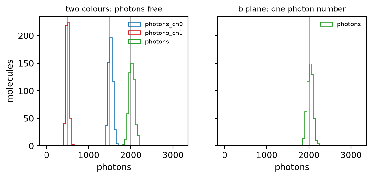
 , the calibrated PSF of that half at the molecule's position and height, scaled to
  photons, on a background
  . x and y reach the secondary half through the transformation, exactly as in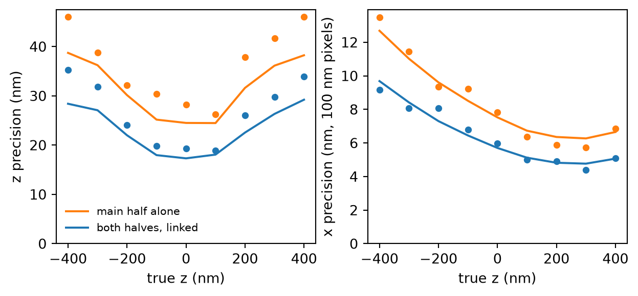
 . Because the fitted height enters both halves' models, the photon split is measured with the PSF of the right height in each half; the colour does not drift with z.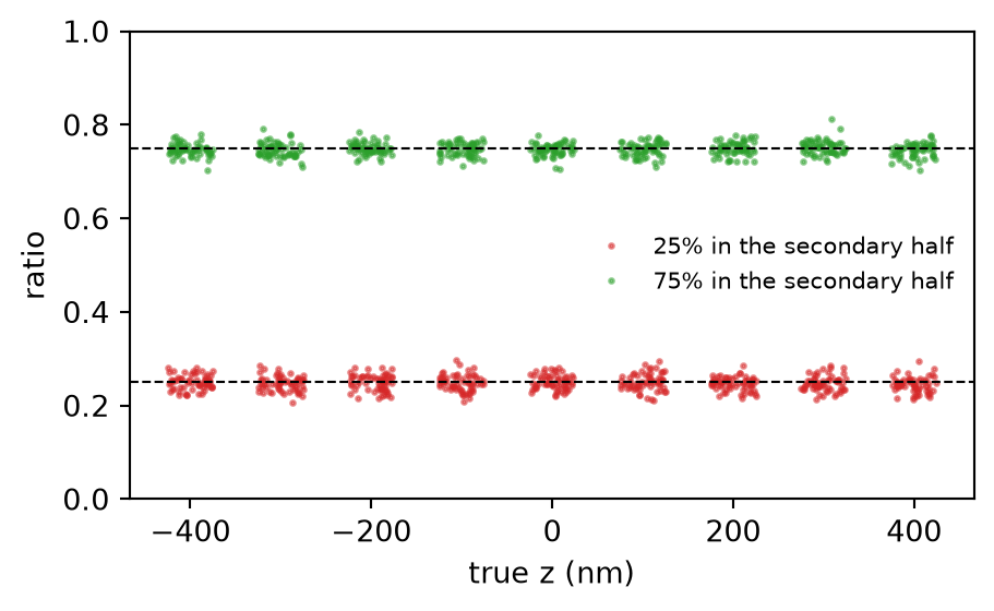
 of the ROI of half
  ,
,
 the cubic spline of half
  ,
,  the linked position in the main ROI, and
  the same position seen through the link:
  , with
  the local scale of the transformation and
  the sub-pixel remainder of cutting the partner ROI at a whole pixel (and the same for y). z has factor 1 and offset 0 in both halves; the calibration's two PSFs are checked on loading to have the same grid, plane spacing and focal plane, and the fit refuses them otherwise. By default the fitted vector is
  , seven numbers for the ten of two separate fits. The likelihood, the Levenberg-Marquardt steps and the Cramér-Rao bound are those of
  . The information about z is summed over both ROIs: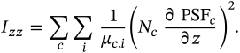
 's signal is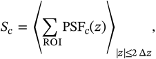
 photons, so a low background never makes it negative. Before version 4 the PSFs were not clipped but lifted: a constant was added to every pixel, large enough to prove the spline positive everywhere. That constant was the worst noise dip anywhere in the volume – 11% of a bright half's signal and 40% of a half with a fifth of the light, from 9 beads – and the fit's background took it: the photons survived, but the fitted background read low by the photons times the constant, and at a photon per pixel it sat on its floor.
 (
( ), half
  's model is
  when the photons are linked, and
  when they are free. What is reported is
 : the split is the one the PSFs carry, the beads', and linked
  . A photon ratio
  (secondary over main photons) sets
  , which splits the one photon number as
  says, and
  is still the total. On simulated beads with a fifth of their light in the secondary half, a dye with a quarter comes back at a
  , and the partner ROI is evaluated about its centre. The calibration stores the secondary PSF in the camera's own orientation, so no image is flipped.
 rather than a flipped image.
 , the colour
 is what is stored, and a linked fit with no ratio given takes the beads' split and reports the total.