Estimate drift from the selected localizations with COMET and subtract it from all of them.
What it does
Over a long acquisition the sample drifts by tens to hundreds of nanometres, and every localization is off by however far it had moved in its frame (the RCC page says more about where drift comes from and what it does to the image). COMET (Reinkensmeier et al. 2026) measures that drift from the localizations themselves – no beads, no fiducial markers – and subtracts it.
It does not make images. It asks a simpler question of the localizations directly: if the drift were known and taken out, a molecule seen early and the same structure seen late would sit on top of each other. So COMET looks for the drift curve that makes localizations from different times overlap as much as possible, and moves every localization by that curve.
Use it on fixed samples: anything that moves by itself is taken for drift. It needs a few thousand localizations in the selection at the least (it warns below 5000), and does better with many more. The drift is estimated from the selection – the filtered localizations, in the ROI if there is one – and subtracted from every localization of the table, so a clean filter (bright, well-fitted localizations) helps the estimate and costs the corrected table nothing.
In the comparisons made while it was developed, COMET was slightly the more precise of the two drift plugins, but it can take minutes where RCC takes seconds, and on a large dataset much longer. It says what a run will cost before it starts. The two share no code and almost no assumptions, so running both is a useful second opinion.
How it works
1. Blinks become molecules. A fluorophore that is on for five frames gives five localizations of the same molecule. They are first linked into one, at their precision-weighted mean position (group blinks). This removes the densest, shortest-range pairs of localizations, which makes the estimate much faster, and stops one bright molecule from counting as five independent measurements.
2. Neighbours. Every pair of localizations closer than max drift is found once, at the start. Only these pairs are ever compared: two localizations further apart than the largest drift cannot be the same structure seen at two times.
3. Overlap. Each localization is treated as a small Gaussian blob of width . For a trial drift curve, every localization is moved back by the drift of its own frame, and the overlap of each pair of blobs is added up. The overlap is largest when the drift curve is right, because then localizations of the same structure land on top of each other whatever time they were recorded at.
4. Coarse to fine. With small blobs the overlap has many small peaks, and an optimiser started far from the answer would stop at the nearest one. So the search starts with wide blobs, a third of max drift, where the overlap has one broad maximum near the answer, and narrows them by a factor 1.5 at a time down to target sigma, each step starting from the last one's answer.
The overlap between the first and the last 1000 frames of a simulated acquisition, as the last ones are shifted in x (the other axes held at their true values). At every width the maximum sits at or near the true drift between the two (dashed); wide blobs give a broad hill that is easy to climb from far away, narrow ones a sharp peak that pins the answer down.
5. A smooth curve in time. By default (fit spline) the drift is a smooth curve with one adjustable point every knot spacing frames (2000), and the overlap is maximised over those points directly. Every localization is moved by the drift of its own frame; there are no time windows. Drift is slow creep, so a few tens of numbers describe an acquisition of tens of thousands of frames, and each is constrained by all the localizations near it in time.
With fit spline off, the method is COMET as published: the acquisition is cut into time windows (window size, 500 frames by default), one drift is fitted per window, and a curve through the windows' values gives the drift of every frame. This follows faster changes and can check each window (quality control), at the price of a noisier curve.
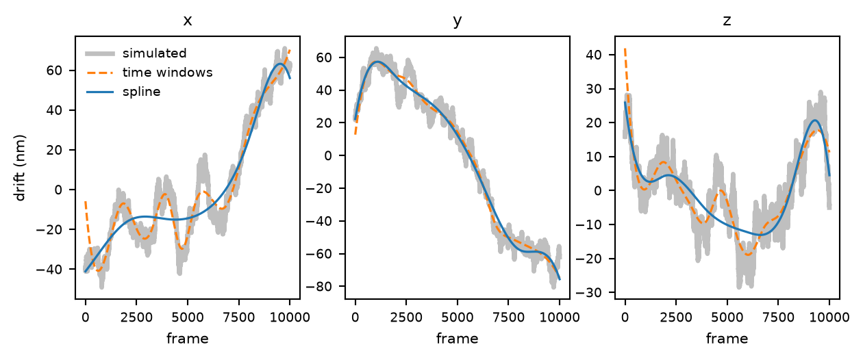
The drift estimated from the simulation, against the drift that was put in (grey, with the frame-to-frame jitter of the simulation). The spline at its default 2000-frame knots (blue) follows the slow course of the drift and smooths over wiggles shorter than its knot spacing; the time-window fit (orange, dashed) follows more of them and is noisier. Only differences between frames are measured, so the curves are compared after removing their mean.
6. Correcting. The drift of each frame is subtracted from x_nm, y_nm and z_nm (or the pixel columns) of every localization in that frame, whether or not it was selected.
Before it starts, the plugin estimates in a fraction of a second how long the run will take and how much memory it needs. Both follow from the number of neighbour pairs, which grows with the square of the number of localizations and steeply with max drift. If the answer is more than five minutes, or more than half the computer's memory, it asks first, and offers an alternative: RCC over a few time windows to take out the bulk of the drift in seconds, then COMET within 50 nm of what is left.
In detail
The cost. With the position of localization (x, y and z, with z zero for a 2D table), its frame and the drift, the overlap is
summed over the pairs with in the uncorrected positions, the max drift. The exponent is the overlap of two Gaussians of width each, which is a Gaussian of variance in their separation. The pair list is built once with a KD-tree and not updated as the drift changes, so must be at least as large as the drift between any two times: a pair that starts further apart is never seen. does not change when the same constant is added to the drift of every frame, so only differences are determined.
and its gradient are computed by a compiled, multithreaded kernel and minimised with L-BFGS-B, stopping when the relative change of the cost falls below ftol (; the gradient tolerance is ), with every parameter bounded to . With approximate kernel on, pairs further apart than after correction are skipped: each contributes less than of a coincident pair, and once is small they are most of the pairs.
The spline. With frames and knot spacing , the drift in each axis is a clamped cubic B-spline
with its knots evenly spaced over frames to . The optimiser's variables are the coefficients ; the kernel returns the gradient with respect to the drift of every frame, and the chain rule to the coefficients is one sparse matrix product. A B-spline cannot overshoot its coefficients, so the curve does not ring between knots the way an interpolating spline through noisy estimates can. A spline penalty adds per axis to the cost.
The widths are (default ), then , one full L-BFGS-B at each, ending with the one at : with the defaults 100, 67, 44 and 30 nm. The spline fit always runs on the CPU and always uses the cutoff.
Time windows (fit spline off). The windows are, by window unit: window size consecutive frames that contain localizations; or frames accumulated until a window holds at least window size localizations; or window size windows, each with about the same share of the localizations. Each window has one drift vector , and a localization's is that of its window. max locs / window keeps a random subset of each window. The width schedule is COMET's own: after each successful L-BFGS-B at width , the run stops if and the median squared change of the parameters over that step was larger than over the step before (or nm); otherwise is divided by 1.5. So it can end below target sigma. Before each step the window drifts are smoothed with a running mean over smoothing windows. Finally a curve through the windows' values, placed at the mean frame of each window's localizations, gives every frame: a cubic spline (cubic) or a Catmull-Rom spline, which is held at the second and second-to-last window's value beyond them.
Quality control (time windows only). After the fit, each window's overlap with its neighbours in other windows is computed with the fitted drift, , and with none, , both per pair. A window whose lift is at most min lift is discarded, and the curve through the remaining windows bridges it.
Two passes.Two stage runs the estimate on grouped localizations, subtracts it, and then runs it again ungrouped with max drift set to fine radius, starting at and ending at ; the two drifts add. RCC first runs RCC over RCC windows windows (grouping as set here), subtracts it, and runs COMET on what is left; again the two add. In both, the second pass searches a small radius, which is what makes it fast. The fit in each pass is the one asked for, the spline or the time windows.
Compared with the paper.Reinkensmeier et al. 2026 present COMET as working directly on 2D or 3D localizations and following drift with a finer time resolution than image cross-correlation. The default here gives some of that time resolution up on purpose: the drift is a smooth B-spline with a coefficient every 2000 frames, not one value per time window, which was less noisy on a real dataset. fit spline off is the time-window fit of the paper's software; Differences from COMET and SMAP lists the other changes.
The cost estimate. The pairs within are counted with a KD-tree on a fixed random sample of at most 60 000 of the selected localizations and scaled by . With grouping on, a stretch of frames from the middle of the acquisition is grouped first, and the fraction it keeps is the fraction the whole table is expected to keep. From the pair count , the time is , plus 0.3 µs per localization of the table, with cost evaluations per width in the schedule above; the memory is 24 bytes per pair. The constants were measured on one computer, so the answer is an order of magnitude, and it is only used to decide whether to ask.
Parameters
The ones shown without more are the ones worth looking at. Several settings under more apply only to the time-window fit and are ignored while fit spline is on; their tooltips say so.
setting
default
what it does
window unit(more) segmentation_mode
frames
What window size counts; time-window fit only. Choices: frames; localizations; windows
window size segmentation_var
500
Frames or localizations per time window, or the number of windows; time-window fit only.
A window must hold enough localizations to show the structure – a few thousand is a good target – and the acquisition must give at least a few tens of windows. With window unit set to localizations, windows get longer as the sample bleaches.
at least 1
max drift max_drift_nm
300 nm
The largest drift expected; also the radius within which localizations are paired.
The setting that decides the running time. Set it to what the stage actually drifts over the whole acquisition, not a safe-looking round number: the pair count, and with it the time and memory, grows steeply with it. Too small, and the drift beyond it cannot be found at all. RCC, or a first run with grouping, is a quick way to find out how large the drift is.
at least 1 nm
target sigma target_sigma_nm
30 nm
The finest width of the overlap Gaussian, where refinement stops.
Smaller sharpens the last step, but the overlap then has more small maxima for the optimiser to stop in. The time-window fit can end below it (see In detail).
at least 0.1 nm
initial sigma(more) initial_sigma_nm
auto
The width the refinement starts from; auto: a third of max drift.
It must be wide enough that the overlap has a single maximum within reach of zero drift, which is why it scales with max drift.
smoothing(more) boxcar_width
1 windows
Running mean over this many windows between refinement steps; 1 is none; time-window fit only.
A running mean over windows also flattens real, fast drift.
at least 1 windows
interpolation(more) interpolation
cubic
The curve from the window estimates to every frame; time-window fit only. Choices: cubic; catmull-rom
max locs / window(more) max_locs_per_segment
auto
A random subset of at most this many per window; auto: all; time-window fit only.
Fewer per window is roughly quadratically faster and less precise; on real data 2000 per window was ten times faster and moved the drift by 2.5 nm rms. The subset is drawn with a fixed seed per window, so a run repeats exactly.
at least 1
ftol(more) optimizer_ftol
1e-07
Relative change of the cost at which the optimizer stops.
COMET's own tolerance is about ; changed the drift by about a tenth of a nanometre on real data for less than half the cost evaluations.
approximate kernel(more) approximate_kernel
on
Skip pairs more than 6 sigma apart; the spline fit always does.
ftol coarse(more) optimizer_ftol_coarse
auto
Ftol for the steps above the target sigma; auto: ftol; time-window fit only.
Loosening it is measured to be a bad trade: faster, but the early steps can land in the wrong maximum, and the fine steps cannot undo that.
backend(more) backend
auto
Where the cost is computed; auto: the fastest available; time-window fit only. Choices: cuda; torch; cpu
quality control(more) quality_control
off
Discard time windows whose fit does not beat no correction; needs fit spline off.
Useful for spotting a window that failed. The spline fit has no windows, and the run refuses the combination.
min lift(more) min_lift
0
How much a window's fit must improve its overlap over no correction to be kept.
0 keeps every window whose fit is better than no correction at all.
group blinks group
on
Link the localizations of one blink into one before estimating.
Grouping made a real estimate 20 to 35 times faster. On real data it also gave a less noisy drift curve, because the repeated localizations of one molecule are not independent measurements.
group radius(more) group_dx_nm
50 nm
How close localizations in consecutive frames must be to be linked.
group gap(more) group_dt
1 frames
How many dark frames a blink may skip.
two stage(more) two_stage
off
A grouped pass, then an ungrouped one within fine radius.
It suits a large dataset where a single ungrouped pass is slow: the grouped pass gets within a few nanometres, and the ungrouped pass refines that over a small radius.
fine radius(more) two_stage_radius_nm
30 nm
The max drift of the second, ungrouped pass.
Well above what the first pass leaves, which is a few nanometres.
RCC first(more) rcc_prepass
off
Correlate rendered time windows to take out the bulk of the drift, then run COMET over a small max drift.
It is the lever when the estimate would otherwise take hours: RCC's cost does not depend on how far it looks, COMET's does.
RCC windows(more) rcc_prepass_windows
10
The time windows RCC correlates. at least 2
RCC max drift(more) rcc_prepass_max_drift_nm
auto
Auto: RCC's own default.
When the plugin offers RCC first before a long run, it puts the max drift that was asked for here and uses 50 nm for COMET.
fit spline spline
on
Fit the drift as a smooth curve in time rather than one value per time window.
knot spacing spline_knot_frames
2000 frames
Frames between the spline's coefficients.
2000 frames was the best choice on a real 46 000-frame dataset: finer knots were noisier without being sharper, and there was no sign of over-smoothing up to 4000. Drift that changes faster wants a smaller spacing.
at least 10 frames
spline penalty(more) spline_penalty
0
Extra penalty on the curve's bending; 0 is none.
Rarely needed: the knot spacing already sets how smooth the curve is. On real data a large penalty flattened genuine early drift rather than removing an artefact.
correct z use_z
auto
Auto: if the table has z.
Output
The table, with the drift subtracted from the position columns of every localization. The run is recorded in the file's history.
The drift curve, x, y and z against frame (the Plot button); an axis with no drift at all is not drawn. It is saved with the file and drawn again when it is reopened.
The text gives the range of the drift in x, y and z, and with quality control the time windows that were discarded.
A good result is a smooth curve of plausible size, a few hundred nanometres at most, and an image that is visibly sharper after correction. A curve that sits flat at twice max drift has run into the optimiser's bound, and max drift was too small. Sharp excursions that come straight back usually mean the data at that time had too little to go on: group blinks, filter more cleanly, or compare with RCC.
Differences from COMET and SMAP
SMAP has no COMET. Its nearest relative there is the DME drift correction, which also works on the localizations rather than on images.
The estimator is COMET 1.1.0 (github.com/gpufit/Comet), vendored with its cost function and optimiser. Around it, this plugin differs from upstream COMET in these ways:
The spline is the default. Upstream COMET fits one drift per time window and interpolates. Here the drift is fitted directly as a B-spline in time, with COMET's cost. On a real dataset, both grouped, its noise was 0.8-1.0 nm against the time-window fit's 1.3-1.7 nm.
Grouping first, by default, which COMET does not do.
Quality control has a different criterion: upstream discards a window whose overlap does not beat its no-drift overlap by at least the standard deviation of the no-drift overlap across windows. On a bleaching sample that spread mostly measures the falling density, and flagged 90 of 92 windows on one dataset. The lift divides the density out.
Two passes and RCC first are additions.
References
Reinkensmeier L, Aufmkolk S, Farabella I, Egner A, Bates M. Cost-function optimized maximal overlap drift estimation for single molecule localization microscopy. bioRxiv (2026), preprint. COMET, the method used here. doi:10.64898/2026.03.27.714864
Cnossen J, Cui TJ, Joo C, Smith C. Drift correction in localization microscopy using entropy minimization. Opt Express 29, 27961 (2021). DME, the localization-based method in SMAP. doi:10.1364/OE.426620
Wang Y, Schnitzbauer J, Hu Z, et al. Localization events-based sample drift correction for localization microscopy with redundant cross-correlation algorithm. Opt Express 22, 15982 (2014). RCC, used by RCC first. doi:10.1364/OE.22.015982
 . For a trial drift curve, every localization is moved back by the drift of its own frame, and the overlap of each pair of blobs is added up. The overlap is largest when the drift curve is right, because then localizations of the same structure land on top of each other whatever time they were recorded at.
 a third of max drift, where the overlap has one broad maximum near the answer, and narrows them by a factor 1.5 at a time down to target sigma, each step starting from the last one's answer.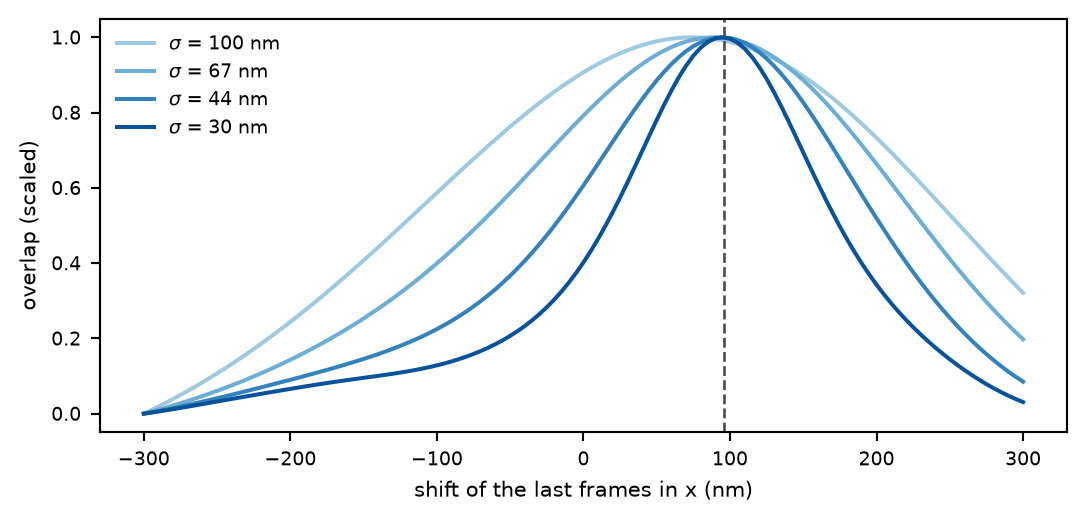
 the position of localization
  (x, y and z, with z zero for a 2D table),
  its frame and
  the drift, the overlap is
 in the uncorrected positions,
  the max drift. The exponent is the overlap of two Gaussians of width
  each, which is a Gaussian of variance
  in their separation. The pair list is built once with a KD-tree and not updated as the drift changes, so
  must be at least as large as the drift between any two times: a pair that starts further apart is never seen.
  does not change when the same constant is added to the drift of every frame, so only differences are determined.
 and its gradient are computed by a compiled, multithreaded kernel and minimised with L-BFGS-B, stopping when the relative change of the cost falls below ftol (
 ; the gradient tolerance is
  ), with every parameter bounded to
  . With approximate kernel on, pairs further apart than
  after correction are skipped: each contributes less than
  of a coincident pair, and once
  is small they are most of the pairs.
 frames and knot spacing
  , the drift in each axis is a clamped cubic B-spline
 to
to  . The optimiser's variables are the
  coefficients
  ; the kernel returns the gradient with respect to the drift of every frame, and the chain rule to the coefficients is one sparse matrix product. A B-spline cannot overshoot its coefficients, so the curve does not ring between knots the way an interpolating spline through noisy estimates can. A spline penalty
  adds
adds  per axis to the cost.
 (default
  ), then
  , one full L-BFGS-B at each, ending with the one at
  : with the defaults 100, 67, 44 and 30 nm. The spline fit always runs on the CPU and always uses the
  cutoff.
 has one drift vector
  , and a localization's
  is that of its window. max locs / window keeps a random subset of each window. The width schedule is COMET's own: after each successful L-BFGS-B at width
  , the run stops if
  and the median squared change of the parameters over that step was larger than over the step before (or
  nm); otherwise
  is divided by 1.5. So it can end below target sigma. Before each step the window drifts are smoothed with a running mean over smoothing windows. Finally a curve through the windows' values, placed at the mean frame of each window's localizations, gives every frame: a cubic spline (cubic) or a Catmull-Rom spline, which is held at the second and second-to-last window's value beyond them.
 , and with none,
  , both per pair. A window whose lift
  is at most min lift is discarded, and the curve through the remaining windows bridges it.
 , starting at
  and ending at
  ; the two drifts add. RCC first runs
  are counted with a KD-tree on a fixed random sample of at most 60 000 of the selected localizations and scaled by
  . With grouping on, a stretch of frames from the middle of the acquisition is grouped first, and the fraction it keeps is the fraction the whole table is expected to keep. From the pair count
  , the time is
  , plus 0.3 µs per localization of the table, with
  cost evaluations per width in the schedule above; the memory is 24 bytes per pair. The constants were measured on one computer, so the answer is an order of magnitude, and it is only used to decide whether to ask.
 ;
;  changed the drift by about a tenth of a nanometre on real data for less than half the cost evaluations.