Gaussian 2D

Localize · version 2 · has a preview

Detect and fit with a free-width Gaussian PSF: x, y, photons, sigma.

What it does

This is where a localization table comes from. It reads the raw camera frames of an acquisition, finds the single fluorophores that are on in each frame, and fits each one with a model of its image – a 2D Gaussian whose width is fitted too – by maximum likelihood (Smith et al. 2010), with the Levenberg-Marquardt fitter of Li et al. 2018, to get its position with a precision far below the size of a pixel. The result is one row per fluorophore per frame: x, y, photons, background, the PSF width, and how precisely each is known.

Use it for 2D data. For 3D data from an astigmatic or otherwise engineered PSF use Spline 3D with a bead calibration; for two channels on one camera, the 2C fitters.

The camera matters: the fit works in photons, so the conversion from the camera's counts (ADU) to photons must be right, or every photon count and every precision is off by the same factor. These values come from the file's metadata or the camera database where possible; check them in the camera section. Preview runs detection on one frame and shows it, which is the way to set the detection threshold.

How it works

The work is done in five steps, each a part of the settings.

1. Counts to photons. A camera reports counts (ADU), which are photons after subtracting the offset and multiplying by the conversion (electrons per count; for an EMCCD, also dividing by the EM gain):

2. Finding candidates. The image is smoothed to suppress noise and the smooth background is subtracted, with a difference of Gaussians: a Gaussian of the PSF's width (filter sigma) minus one 2.5 times wider. A spot then stands out as a bump on a flat floor. Every pixel brighter than all eight of its neighbours is a local maximum, and those above a threshold (cutoff) are candidates.

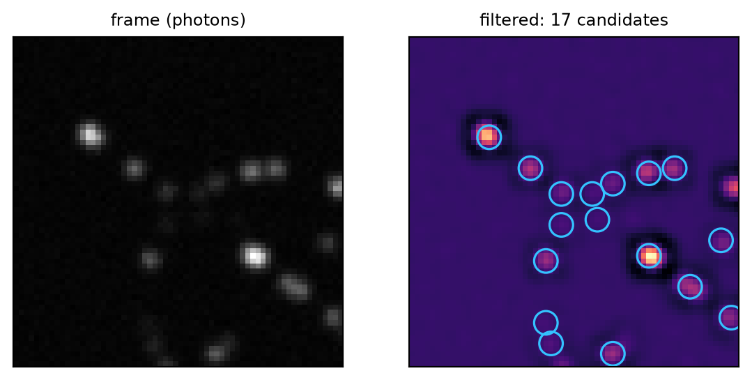
One simulated frame, in photons (left), and after the difference-of-Gaussians filter (right), with the candidates above the dynamic cutoff circled.

The dynamic cutoff adapts to each frame by itself. Most local maxima of the filtered image are noise, and their values form a distribution; the cutoff is set above it,

with and the 20th and 80th percentiles of the maxima of that frame, and the cutoff value (1.7). The fraction is a robust measure of the spread of the noise, so the cutoff is " noise widths above the typical maximum" whatever the background. The absolute cutoff is a fixed number, in photons of the filtered image. Lower values find dimmer molecules and more noise.

3. Cutting ROIs. A small square (ROI size, 13 pixels) is cut around each candidate. A candidate too close to the edge of the image for its ROI to fit is dropped rather than fitted off centre.

4. The fit. Each ROI is compared with a model of what a single emitter looks like: a Gaussian of width , integrated over each pixel, with photons, at position , on a flat background per pixel,

The five parameters are those that make the observed pixels most probable, given that each pixel's photon count is Poisson distributed around – the maximum likelihood estimate. This is the best that can be done with the data: it makes use of every photon, and weighs each pixel by how noisy it really is.

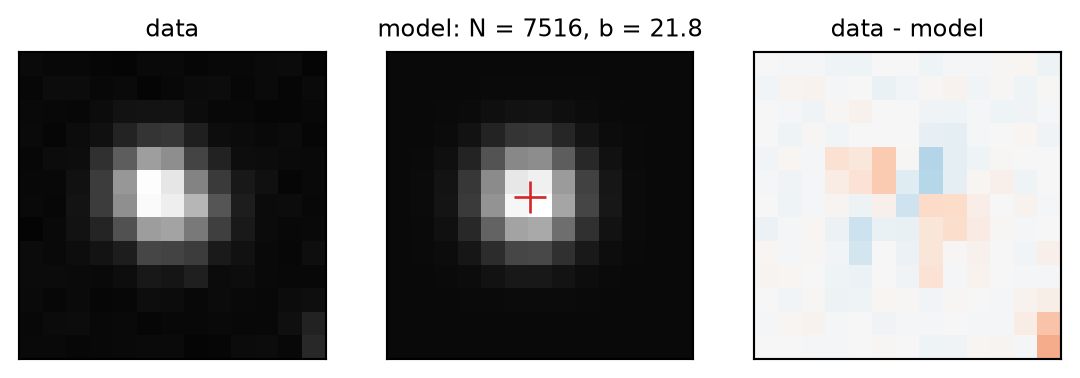
One ROI from the frame above: the data, the fitted model, and what is left over. A good fit leaves only noise.

The likelihood is maximised iteratively, with the Levenberg-Marquardt method (details below), from a start at the ROI's centre of mass.

5. Precision, and the table. The fit also says how well it could possibly have done. From the model, the Cramér-Rao lower bound (CRLB) is the smallest variance any unbiased estimate of each parameter can have, and a maximum likelihood fit reaches it. Its square root is written as the precision of each localization (x_err, y_err and their root mean square xy_err, photons_err, ...). It is what the precision histograms of Localization Statistics show and what renderers blur by.

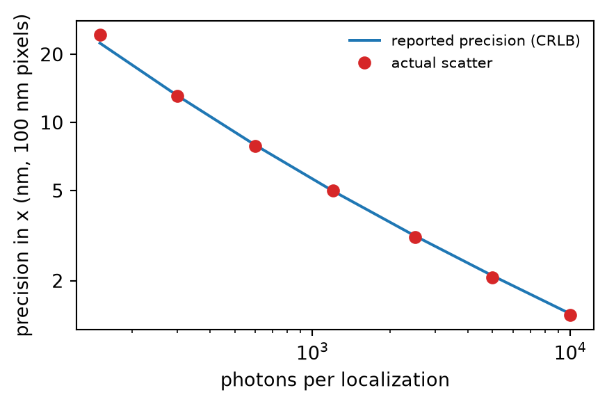
The fitter reaches the bound. Thousands of spots simulated with known positions (1.3 pixel PSF, 10 background photons per pixel) and fitted: the scatter of the fitted positions about the truth (dots) against the precision the fitter reported (line), both falling as .

Finally positions are converted to nanometres with the pixel size, fits that failed (a position or photon count that is not a number) are dropped, and the table is saved as <acquisition>_locs.hdf5 next to the data.

In detail

The likelihood. For Poisson pixels, maximising the likelihood is minimising the deviance

which is zero for a perfect model and grows with every pixel it gets wrong. Its gradient and curvature with respect to the parameters come from the derivatives of the model, which for a pixel-integrated Gaussian are in closed form.

Levenberg-Marquardt. Each iteration solves for a step with the curvature matrix – here the expected information

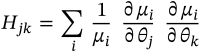
– with its diagonal enlarged by a factor . A small is a Newton step, a large one a short step downhill. shrinks after a step that lowered the deviance and grows after one that raised it by more than half; a step that went that far wrong is undone. Each parameter's step is also capped (one pixel for the position, at first), and the cap is halved whenever the step reverses direction. The fit stops when the deviance changes by less than one part in a million, or after iterations steps.

The start. Position: the centre of mass of the ROI. Background: the mean of its border pixels. Photons: the brightest pixel above background, times . Width: start sigma, . During the fit , and half the ROI. The position is not held inside the ROI: a fit that runs away is visible, and max fit distance rejects those that end further than that from their candidate.

The CRLB. The Fisher information is the matrix above at the fitted parameters; its inverse is the covariance of the best possible unbiased estimate, and its diagonal the CRLB; x_err is :

With no background it is simply per axis, with the PSF's width widened by the pixel size ; background adds to it, the more so the dimmer the spot. That is why the precision is quoted with the photons: they set it.

EMCCD cameras. Electron multiplication doubles the variance of the signal (the excess noise factor, 2 for high gain), so the pixels are no longer Poisson. The photons are divided by 2 before the fit, which makes them Poisson again with half the counts, and the fitted photons and background are multiplied by 2 afterwards. The precision then correctly reflects the extra noise.

Read noise. A camera without EM gain – an sCMOS – adds Gaussian read noise, about one electron per pixel, to the Poisson counts, and a Poisson likelihood cannot take it: a count read as negative is treated as none, and at a photon or two of background the background comes out too high. So the read noise's variance is added to every pixel of the data and of the model before the fit (Huang et al. 2013), which makes the likelihood Poisson again to a good approximation and weighs each pixel by ; it is taken off the fitted background afterwards. read noise sets : by default 1 electron without EM gain and 0 with it, since the gain leaves the read noise a fraction of an electron. On simulated spots at half a photon of background and one electron of read noise, the background comes back at 0.53 rather than 0.74. The variance is one number for the whole chip; an sCMOS's varies from pixel to pixel (0.7 to 1.4 electrons), which a variance map would capture and this does not.

Quality of the fit. logl is the log-likelihood of the fit and logl_rel the same per pixel of the ROI, so that it can be compared between ROI sizes. A spot that is not one emitter (two overlapping, or a bright speck of something else) fits badly, and filtering on logl_rel removes most of them.

Speed. Detection runs on blocks of frames; ROIs are collected and fitted in batches (ROIs per fit), on all cores, in C++. Reading the file runs in the background while the previous block is processed.

Compared with the papers. The fit and its CRLB are those of Smith et al. 2010, and the steps those of Li et al. 2018, with these differences:

• Smith et al. fit four parameters, with the PSF width measured beforehand and held fixed; here the width is a fifth parameter, started at start sigma.
• They leave out read noise, negligible on an EMCCD at high gain; here its variance is added for an sCMOS (Read noise above).
• Li et al. drop the model's second derivatives from the curvature, which leaves as each pixel's weight; here the data in it is replaced by the model – the expected information above – so that a background near zero no longer shrinks the steps to nothing. They raise tenfold after any step that does not lower the deviance; here only after one that raised it by more than half.

Parameters

Output

The table, with one row per fitted spot:

column	meaning
frame	the camera frame
x_nm, y_nm	the position
photons, background	, and per pixel
x_err_nm, y_err_nm, xy_err_nm	the precision (CRLB)
photons_err, background_err	their CRLB
sigma_nm	the fitted PSF width (sigma_x_nm, sigma_y_nm if elliptical)
logl, logl_rel	the log-likelihood, and per pixel
peak_x_pix, peak_y_pix	the candidate the ROI was cut around
iterations	how many steps the fit took

The file also records the camera, the settings and the software version, so it can always be told how a table was made.

The camera frames. The file also keeps a few of the frames the table was fitted from, in photons (counts minus offset, times the conversion): first the average of every frame fitted, then the first fitted frame, then the rest spaced evenly up to the last one, as many as raw frames asks for, each with its frame number – the same number as in frame. In the Render tab they are a source of an image layer, placed in the table's coordinates, so they lie under the localizations: whether a structure is really there, where the cell edge is, or whether the focus was lost can be checked without the original stack. The average is the one to start with; a localization of frame 17 should sit on a spot in frame 17.

Differences from SMAP

Based on SMAP's fit_fastsimple workflow and its MLE_GPU_Yiming fitter (Ries 2020). The main changes:

• The curvature used for the steps is the expected (Fisher) information rather than the observed one, and the background starts at the ROI's border rather than its minimum. Both have the same answer; together they let a fit at very low background converge instead of sticking at zero background.
• The position is not clamped to the centre of the ROI; runaway fits are removed by max fit distance instead.
• Read noise is one variance for the whole chip, added to data and model (1 electron by default without EM gain); SMAP's sCMOS mode reads a per-pixel variance map instead, which is not ported.
• No Anscombe transform or background estimation before detection.
• Raw frames by number, not by spacing. SMAP's CameraConverter keeps every diffrawframes-th frame after the average; here a number of frames is kept, spaced evenly over the fitted range, so that a long acquisition does not fill the file with them.

References

• Smith CS, Joseph N, Rieger B, Lidke KA. Fast, single-molecule localization that achieves theoretically minimum uncertainty. Nat Methods 7, 373 (2010). doi:10.1038/nmeth.1449 – the maximum likelihood fit and its CRLB.
• Li Y, Mund M, Hoess P, et al. Real-time 3D single-molecule localization using experimental point spread functions. Nat Methods 15, 367 (2018). doi:10.1038/nmeth.4661 – the Levenberg-Marquardt implementation this one follows.
• Mortensen KI, Churchman LS, Spudich JA, Flyvbjerg H. Optimized localization analysis for single-molecule tracking and super-resolution microscopy. Nat Methods 7, 377 (2010). doi:10.1038/nmeth.1447 – the precision formula, and the excess noise of EMCCDs.
• Huang F, Hartwich TMP, Rivera-Molina FE, et al. Video-rate nanoscopy using sCMOS camera-specific single-molecule localization algorithms. Nat Methods 10, 653 (2013). doi:10.1038/nmeth.2488 – the read noise's variance added to data and model.
• Ober RJ, Ram S, Ward ES. Localization accuracy in single-molecule microscopy. Biophys J 86, 1185 (2004). doi:10.1016/S0006-3495(04)74193-4 – the Fisher information limit.
• Ries J. SMAP: a modular super-resolution microscopy analysis platform for SMLM data. Nat Methods 17, 870 (2020). doi:10.1038/s41592-020-0938-1