Calibrate transform

Analysis › Register · version 2 · has a preview

Measure the transformation between the two halves of a split frame from localizations fitted over the whole frame: no initial shift, no magnification and no split position needed.

What it does

A two-colour splitter images the sample twice, side by side on one camera: each half of the chip sees the same field through a different filter. The two images never lie exactly on top of each other. The second is shifted, slightly turned and slightly magnified, and at the corners of the field the difference is several pixels. To combine the two halves – to fit each molecule in both, as Gaussian 2D 2C does – the program needs the transformation that maps a position in one half onto the same position in the other.

This plugin measures that transformation from localizations, without beads. In a ratiometric experiment every molecule is imaged in both halves at once. Fit the whole frame with a plain Gaussian 2D fit, ignoring the split, and each molecule shows up twice in the same frame. The plugin finds those pairs, and fits the map that takes one partner onto the other.

It needs no starting values: not the shift, not the magnification, and not where the chip is split. It also detects whether one half is mirrored. What it needs is a table with a frame column and positions that can be put back into camera pixels, and enough molecules seen in both halves: a few hundred pairs at the least, from frames spread over the movie.

The 2C fit can do this step itself, on the first frames of the movie (calibrate from this movie). Run it here to see what it found before trusting it, or to save a transformation for movies too sparse to register on.

How it works

1. Positions in camera pixels. A transformation is a property of the camera, so it is measured in chip pixels. A table in nanometres is converted back with the pixel size the fit recorded. Only the localizations of the current selection are used – the layer's filter and the ROI.

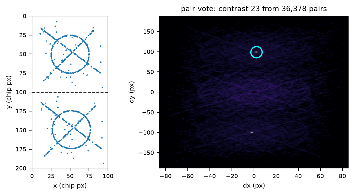
2. The vote. For every two localizations in the same frame, the vector from one to the other is collected. Most of these vectors connect unrelated molecules and point anywhere. But every molecule seen in both halves adds the same vector – the offset between the halves – so over many frames that vector turns up again and again, and stands out in a histogram of all of them as a sharp peak. Its position is the offset, found without any guess. A mirrored half is found the same way on the sum of the coordinates along the mirrored axis instead of their difference. All three possibilities are tried, and the sharpest peak decides the layout.

Left: the simulated localizations on the chip; every molecule of the upper half appears again in the lower one. Right: the vote, the vectors between all localizations of a frame – the ring marks the one offset that thousands of them share.

3. The split. The offset says which way the chip is split (the axis along which the partners are far apart) and gives a first map. The pairs found through it then place the seam between the halves: a localization whose partner lies above it is in the lower half, and the other way round.

4. Pair and fit, twice. First, every localization is paired, frame by frame, with the nearest one where the offset says its partner should be, within coarse matching (20 pixels). The offset is only a shift; the wide tolerance is what lets the pairs still be found when the halves are also turned or scaled. A projective transformation is fitted to these pairs, robustly, so that the chance pairs a wide tolerance lets in are voted out (In detail). Then everything is paired again, this time through the fitted map and within fine matching (1 pixel, or wider if the first fit shows it must be), and the map is fitted again on these clean pairs. The second round is where the accuracy comes from.

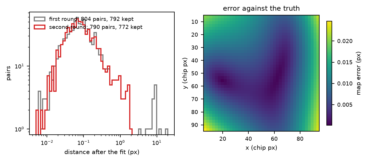
Left: how far the partners of each pair are apart after the fit. The first round, paired within 20 px on the offset alone, lets in chance partners (the tail), which the robust fit rejects; the second, paired through the fitted map, keeps clean pairs only. Right: the error of the final map over the field, against the transformation that was simulated – a hundredth of a pixel, far below the scatter of a single pair.

5. Optionally, a polynomial. A projective map describes a shift, a rotation, a scale, a shear and a tilt of the field, but not the curved distortion a lens can add towards the edges. With transformation set to polynomial, a third-order polynomial is fitted on top of the projective result, the pairs are matched again through it and it is fitted again. It is refused – the projective map is kept, and the reason given – when there are too few pairs or they cover too little of the field, because outside its pairs a polynomial is not to be trusted.

6. Saving. With save transformation, the map, the geometry of the split and what it was measured from are written to a _2ct.h5 file, which the two-colour fit's transformation reads.

In detail

The vote. For each frame, every ordered pair of its localizations gives a feature vector: for an unmirrored layout, or with the sum (or ) on the mirrored axis. Frames are taken in order until 4 000 000 vectors have been collected. The vectors are binned into a histogram with bins of vote bin (2 px), and scored with a difference of Gaussians

being vote smoothing (4 px), so that the sharp peak of the pairs stays and everything broad – short vectors between neighbours in one half, the ridge that one-half pairs draw in a mirrored vote – subtracts away. In an unmirrored vote the 3 bins around zero are left out. The contrast is the peak of over the standard deviation of ; the layout with the highest contrast wins, and the peak is refined to below a bin by the centroid of the counts around it. An unmirrored vote has two equal peaks, and ; the one pointing from the lower to the higher side of the split is taken. For a mirrored vote, whose sign on the other axis matters, both are tried and the one that pairs more localizations is kept.

The mirror line. Reflected about a line at , partners satisfy , so the peak of a mirrored vote is the mirror line itself. It is taken as the split; a residual shift of the mirrored half cannot be told apart from a seam moved by half of it, so for a mirrored layout the split is an estimate, and split position is there to set it.

The seam. Unmirrored, the seam is placed between the 99.9th percentile of the lower side's positions and the 0.1th percentile of the upper side's, each localization sided by where its partner is under the first round's map, paired at the fine tolerance. If the band between the two is wider than 8 pixels, a warning says the split is only known to within it.

Pairing. Two localizations of one frame are partners when each is the other's nearest neighbour and they are within the tolerance, after the secondary half has been mapped into the reference half – so the tolerance is a distance in the reference channel in every round. At most pairs used in the fit (20 000) pairs, drawn at random, go into a fit.

The projective map. With a position in the secondary half and in the reference half,

eight free coefficients, since the nine are fixed only up to a common factor. The linear solution for a set of pairs is the normalised direct linear transform: both point sets are centred and scaled to a root-mean-square distance of from their centre first, which keeps the solve well conditioned (Hartley 1997).

The robust fit, in each round:

RANSAC (Fischler & Bolles 1981): 500 times, four pairs are drawn at random and the map through them is computed; the draw that brings the most pairs within the outlier threshold wins (ties go to the smaller truncated squared error). The map is then refitted on its inliers until the inlier set changes by no more than 0.2% of the pairs, at most 10 times.
A soft-L1 refinement of the eight coefficients on those inliers, minimising over the x and y misfits , with 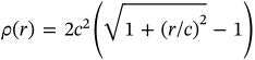– quadratic for small misfits, linear for large ones – and half the dx/dy limit.
A screen: a pair whose misfit in x or in y exceeds the dx/dy limit is dropped, and the map is fitted again, as in 2, on what is left.

The outlier threshold and the dx/dy limit widen with the round's tolerance, to at least a half and a quarter of it: 10 and 5 pixels in the first round, the set values in a tight second round.

Weights. If the table has a precision – xy_err_pix, or xy_err_nm converted with the pixel size it records – a pair's weight is the inverse variance of its separation,

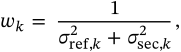
normalised to a mean of one. A dim channel usually brings many poorly localized partners; unweighted, they would outnumber the good ones. RANSAC itself is unweighted: a precise outlier is still an outlier.

The second round's tolerance. With adapt_fine_tolerance on, the second round is widened to 3 times the 98th percentile of how far the first fit misses its own accepted pairs, up to the coarse tolerance. Where a projective map misfits a distorted field, it misfits most at the edges, and a fixed tight tolerance would lose exactly those pairs. If the first fit accepted less than 60% of its pairs, its misfit comes from chance partners rather than distortion, and the tolerance is left alone.

The polynomial. Third order: all 10 monomials with in centred, scaled coordinates, for each of x and y – 20 coefficients. Order three, because radial distortion is cubic in the coordinates, and a quadratic cannot represent it at all. It needs at least 10 pairs per coefficient (200), and the pairs' convex hull must cover at least half of the reference channel's localizations' hull. It is a linear least-squares fit, reweighted 4 times by 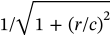against outliers, with a quarter of the tolerance (at least 0.05 px); both directions are fitted, since a polynomial has no closed-form inverse.

The checks. Two warnings are raised on the final pairs: when the median misfit in the outer half of the paired region is more than twice that in the inner half (and above 0.1 px), which means the model does not describe the field; and when the kept pairs cover less than half of the reference channel, which means the map is an extrapolation over the rest.

Parameters

setting	default	what it does
registration – How hard to look, and what is already known.
layout `registration.layout`	detect	How the chip is split; detect votes for all of them and keeps the sharpest. Set it only when detection picks the wrong one: declared, the vote is taken only in the space that layout needs. Choices: detect; right-left; right-left mirrored; up-down; up-down mirrored
main channel `registration.main_channel`	the left or upper half	The half the other is mapped onto, the reference. Choices: the left or upper half; left; right; upper; lower
transformation `registration.model`	projective (8 coefficients)	Projective extrapolates gracefully; the polynomial describes a distorted field far better where the pairs reach, and is refused when they do not reach far enough. Stay with projective unless the residual grows towards the edges of the field (the warning, or the residual panel) and the pairs cover the whole chip. Choices: projective (8 coefficients); polynomial, order 3 (20)
split position `registration.split_position`	auto	Auto: measured from the pairs, in chip coordinates. Worth setting for a mirrored layout, where the pairs cannot place the seam, or when the warning says the two halves leave a wide band without pairs. at least 1 px
vote bin (more) `registration.vote_bin_px`	2 px	The bin of the histogram of pair vectors the offset is voted in. at least 0.1 px
vote smoothing (more) `registration.vote_smooth_px`	4 px	The width of the difference-of-Gaussians filter the vote is scored with. at least 0.1 px
coarse matching `registration.coarse_tolerance_px`	20 px	First pass; must cover the rotation between the channels – 3 degrees over 512 px is 27 px. The first thing to raise if no pairs are found and the halves are strongly rotated. Wider costs more chance pairs, which the robust fit then has to reject. at least 0.1 px
fine matching `registration.fine_tolerance_px`	1 px	Second pass over clean matches only, which is where the accuracy comes from; 0 skips it. One pixel is roughly seven times the residual of a good registration. Much tighter strips the edges of the field; skipping the second round costs a factor of three to seven in accuracy.
adapt fine matching (more) `registration.adapt_fine_tolerance`	on	Widen the fine matching to what the coarse fit misses its own pairs by, when those pairs are clean. See In detail. Off, the second round pairs at exactly fine matching.
minimum pairs (more) `registration.min_pairs`	20	Fewer pairs than this and the registration refuses. at least 4
pairs used in the fit (more) `registration.max_pairs`	20000	At most this many pairs, drawn at random, go into each fit. Tens of thousands of pairs buy no more accuracy than a well-spread twenty thousand. at least 4
outlier threshold (more) `registration.reprojection_threshold_px`	1 px	The robust (RANSAC) fit's inlier radius, at least; it widens with the matching tolerance. at least 0.01 px
dx/dy limit (more) `registration.transform_axis_limit_px`	0.5 px	The largest \|dx\| or \|dy\| a pair may keep after the first fit, at least; it widens with the matching tolerance. at least 0.01 px
save transformation `save`	on	Write it to a file a two-colour fit can read.
file `path`	–	Auto: <name>_2ct.h5 beside the movie the table was fitted from (or the file it was read from). With no source recorded in the table, the automatic name is `channels_2ct.h5` in the working folder. Saving refuses to replace an existing file unless overwrite is ticked.
overwrite (more) `overwrite`	off	Replace a file that is already there.

Output

The text: the layout, where the split is and which half is the main one; how many pairs were kept of how many, from how many localizations and frames; and the residual in x and y, in pixels, with the median misfit in the middle of the paired region and at its edge.
The figure, three panels; the Preview button draws it without writing a file.
The pair vote: a single sharp peak (the ring) against a faint background is a found offset. A smear, or a peak barely above the rest (a low contrast), means the halves were not found.
The residual: where each kept pair lands after the fit, the rejected ones in red. A round cloud a fraction of a pixel wide, about the localization precision, is good; a stretched or split cloud means the map is wrong.
The pairs used: where in the reference half the pairs are. The map is measured only there; anywhere else it is extrapolated, however small the residual.
The file, with save transformation: the projective map (always, also for a polynomial), the geometry of the split, the numbers of the text, the polynomial if one was fitted, and the pairs and the vote for a later look.

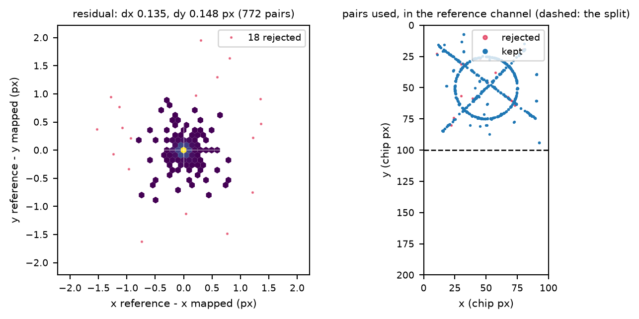
The plugin's residual and coverage panels for the simulated splitter: a round cloud about 0.15 px wide, and pairs over the whole of the upper half.

Differences from SMAP

Based on SMAP's Process/Register/RegisterLocs2 (Ries 2020), whose sequence – a global alignment, then pairing and refitting at a shrinking tolerance – it keeps.

The global alignment. SMAP renders both halves into images (500 nm pixels) and cross-correlates them; the user says where the second half is (target position) and whether it is mirrored, and the split is the middle of the ROI. Here the offset is voted for on the pair vectors themselves, which is the same cross-correlation computed on points, and the layout, the mirroring and the split position are all measured from the pairs. A seam away from the middle of the chip then needs no setting.
The fit. SMAP fits the pairs with MATLAB's fitgeotrans by plain least squares. Here the fit is robust – RANSAC, a soft-L1 refinement and a dx/dy screen – and weighted by the localization precision.
Models. SMAP offers MATLAB's projective, affine, similarity, polynomial and local (lwm, pwl) transformations. Here: projective, or a third-order polynomial that is refused when the pairs do not support it.
Scope. SMAP can register two files (two cameras) and fits a z transformation for 3D data. Here the two channels are the two halves of one chip, in one table, and the map is 2D.
The second round's tolerance follows the first round's misfit instead of a fixed value (SMAP: 1250 nm, then 150 nm).

References

Fischler MA, Bolles RC. Random sample consensus: a paradigm for model fitting with applications to image analysis and automated cartography. Commun ACM 24, 381 (1981). doi:10.1145/358669.358692 – RANSAC, the robust first fit.
Hartley RI. In defense of the eight-point algorithm. IEEE Trans Pattern Anal Mach Intell 19, 580 (1997). doi:10.1109/34.601246 – the normalisation before the linear solve.
Ries J. SMAP: a modular super-resolution microscopy analysis platform for SMLM data. Nat Methods 17, 870 (2020). doi:10.1038/s41592-020-0938-1