 and
and  the cross-correlation
Analysis › Drift · version 1
Estimate drift by cross-correlating rendered time windows (RCC) and subtract it from all localizations.
During an acquisition of many minutes the sample moves by tens to hundreds of nanometres: the stage creeps, the objective warms up, the coverslip settles. Every localization is then off by however far the sample had moved in its frame, and the super-resolved image is smeared by the whole path.
RCC (redundant cross-correlation, Wang et al. 2014) measures that path from the localizations themselves – no beads or fiducial markers are needed – and subtracts it. It cuts the acquisition into time windows, makes an image of each, and asks how far one image has to be shifted to match another. The answer, for every pair of windows, is the drift between them.
Use it on fixed samples. It assumes the structure itself does not change, only where it is, so anything that moves by itself (live cells, diffusing molecules) is taken for drift. It needs enough localizations per window for each image to show structure: a few thousand in the selection at the very least (below 5000 the plugin warns), and many more for a precise curve.
It is the classic method, and fast – seconds, where COMET takes minutes. The two share no code and almost no assumptions, so running both is a useful second opinion on a drift curve.
1. Time windows. The frames are split into a number of equal windows (time windows, 20 by default). Blinks are first grouped, so that a molecule that is on for five frames counts once rather than five times (group blinks).
2. An image per window. The localizations of each window are binned into a 2D histogram with small pixels (15 nm by default).
3. Cross-correlation. For two images and the cross-correlation

is large at the shift  that best lays one onto the other. Its peak is the drift between the two windows. The correlation is computed with Fourier transforms, which is what makes it fast, and the peak is looked for only within max drift of zero. Its position is refined below a pixel by fitting a paraboloid to the few pixels around the maximum.
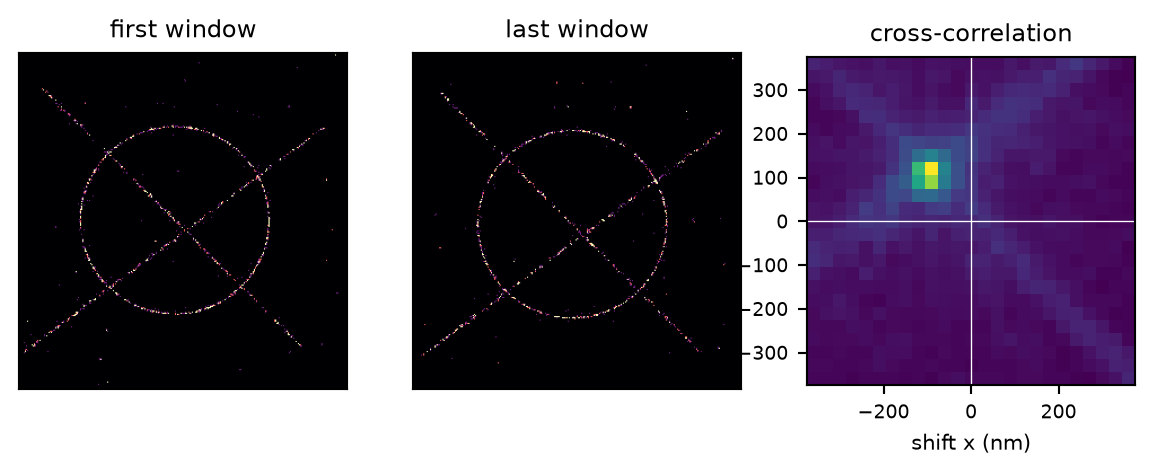
The first and the last time window of a simulated acquisition with drift, and their cross-correlation: the peak sits where the last window has to be shifted to match the first – the drift between them.
4. Every pair, not just neighbours. Correlating only consecutive windows and adding up the shifts would add up their errors too, and one bad correlation would offset everything after it. Instead every window is correlated with every other: with  windows that is
  measurements
  of the difference
  between the drift of two windows, for only
  unknowns. This redundancy is the R in RCC.
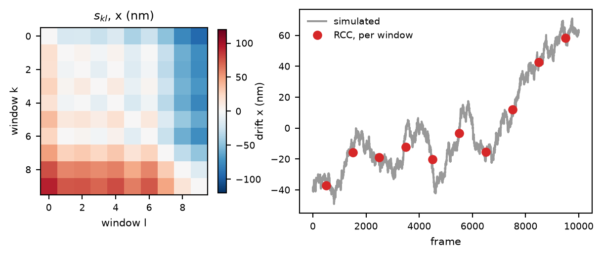
Left: the measured shift in x of every window against every other – one number per pair,  of them. Right: the drift per window that best explains all of them (dots), against the drift that was simulated (line).
5. The least-squares solution. The drift per window is the set of  that fits all pair measurements best. A pair whose correlation peak landed in the wrong place – a window with little structure, a coincidence of shapes – is then outvoted by the others instead of believed. How that is done is under In detail.
6. z, if the table has it. The axial drift is measured the same way, but on z histograms rather than images: the lateral drift is taken out first, the field of view is cut into small tiles (200 nm), each tile's z histogram is correlated between the two windows, and the correlations of all tiles are added up before the peak is found. Tiles matter: a z histogram of the whole field mixes hundreds of structures into a featureless slab with nothing for the correlation to lock onto.
7. Per frame. The drift per window is interpolated to every frame with a smooth curve that does not overshoot between the windows (PCHIP), and subtracted from every localization – of the whole table, not only of the selection it was measured on.
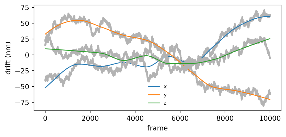
The drift estimated from the simulation (coloured) against the drift that was put in (grey). Only differences between windows are measured, so the curves are compared after removing their mean.
The pair equations. With  the measured shift of window
  against window
  , the drifts
  solve, in the least-squares sense,

Only differences are measured, so the drift is fixed to average zero; the absolute position of the sample over the acquisition is not known and is not needed. x, y and z are solved separately.
Robust weights. The system is solved five times, each time weighting a pair by how well the previous solution explained it. With residuals  and their robust spread
  , a pair's row of the system is multiplied by the Cauchy weight
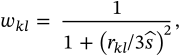
so a pair three robust standard deviations off counts half, and one far off counts almost nothing. The equations are linear in the unknowns, so each pass is a plain linear least-squares solve.
The peak. The correlation is smoothed with a  box before the maximum pixel is picked (the largest pixel of a noisy correlation can sit one off the ridge), then a quadratic surface
  is fitted to the unsmoothed correlation over
  pixels around it,
  the peak fit half-width, and its stationary point is the sub-pixel shift. If the fit is not a maximum or lands outside the patch, the pixel is kept.
The images. The images are padded before the Fourier transform so that the circular correlation does not wrap onto itself within the search range. A field of view wider than max image size pixels is folded back onto itself: the structure repeats, but a shift of the whole is still a shift, and the transform stays bounded.
z. Each tile's z histogram (bins of z bin) has its mean subtracted, so that the correlation follows structure rather than the number of localizations. The sample at zero shift is left out of the peak search and the fit (skip zero shift): anything that sits at the same z in both windows regardless of drift – the same molecule on in both, or localizations piled up at one z by the fitter – would pull the answer towards no drift. The axial peak is searched within max axial drift, which is kept smaller than the lateral range because a z profile is much less structured than an image and a wide range lets the maximum wander.
Compared with the paper. The method is that of Wang et al. 2014: images of time windows, every window correlated with every other, and the drift solved from the redundant set of shifts. The main changes are SMAP's and this code's (Differences from SMAP): blinks are grouped before the images are made, a pair that disagrees with the rest is weighted down by the Cauchy weight above, and z comes from the tiled z histograms.
What limits the precision. The noise of the curve falls with more localizations per window, and rises with more windows (fewer localizations in each); more windows follow faster drift. Twenty windows is a good start for an acquisition of 10 000 to 50 000 frames. If the curve looks noisy, use fewer windows; if it looks like it cuts corners, use more, or COMET.
The ones shown without more are the ones worth looking at; the defaults of the rest rarely need changing.
| setting | default | what it does |
|---|---|---|
time windowsn_timepoints | 20 | How many windows the acquisition is cut into: more follow faster drift, fewer are less noisy. Twenty is a good start for 10 000 to 50 000 frames. A noisy curve wants fewer; a curve that cuts the corners of the real drift wants more. at least 2 |
pixel sizepixelsize_nm | 15 nm | The pixel of the images that are correlated; about the localization precision. Much smaller makes the images sparse and the correlation noisy; much larger blurs the structure the correlation locks onto. at least 1 nm |
z bin (more)z_pixelsize_nm | 5 nm | The bin width of the z histograms. at least 0.1 nm |
max driftmax_drift_nm | 500 nm | The largest drift between any two windows that can be found. Set it above the total drift over the whole acquisition. A larger range costs little, but gives a spurious peak more room. at least 1 nm |
peak fit half-width (more)fit_window | 3 pix | The patch the correlation peak is fitted over, for its sub-pixel position. at least 1 pix |
max image size (more)max_pixels | 2048 pix | A wider field of view is folded back onto itself, to keep the correlation fast. at least 64 pix |
correct zuse_z | auto | Auto: if the table has z. |
group blinksgroup | on | Link the localizations of one blink into one before measuring. It removes the correlation of a molecule with itself in consecutive frames, and makes the estimate faster. |
group radius (more)group_dx_nm | 50 nm | How close localizations in consecutive frames must be to be one blink. |
group gap (more)group_dt | 1 frames | How many dark frames a blink may skip. |
tile (more)tile_nm | 200 nm | The axial pass correlates z histograms in tiles of the field of view this size. at least 1 nm |
tile y (more)tile_y_nm | auto | Auto: square tiles. at least 1 nm |
max axial drift (more)axial_max_drift_nm | 200 nm | How far from zero the axial correlation peak is looked for. Smaller than the lateral range, because the axial correlation is broad and a wide range lets its maximum wander. at least 1 nm |
skip zero shift (more)exclude_zero_lag | on | Leave the zero-shift sample out of the axial peak search. See In detail. |
x_nm, y_nm and z_nm (or the pixel columns) of every localization. The correction is recorded in the file's history and can be undone.A curve that is smooth and plausible (a few hundred nanometres at most, slow changes) is a good sign. A curve that jumps between windows means the correlations had too little to work with: fewer windows, more localizations, or a larger pixel size.
Based on SMAP's Drift/driftcorrectionXYZ (Ries 2020), its finddriftfeature in particular.