Spline 3D

Localize · version 2 · has a preview

Detect and fit with an experimental spline PSF from a bead calibration: adds z.

What it does

This is the 3D fitter. It does what Gaussian 2D does – reads the camera frames, finds the single fluorophores that are on, and fits each one to get its position far below the size of a pixel – but the model it fits is not a Gaussian. It is the measured image of a point source on this microscope, at every height, taken from a bead calibration and interpolated with cubic splines – the method of Li et al. 2018. Because that image changes with the emitter's distance from the focal plane, the fit also tells how far it was: every localization gets a z_nm and a z_err_nm besides x, y and the photons.

The shape has to change with z in a way that tells above from below. The usual way is a weak cylindrical lens in the detection path (astigmatism): the spot is then stretched along one axis above focus, along the other below, and round in between. Any other engineered PSF works as well, as long as the calibration was measured with it – and so do the aberrations of an ordinary objective, which a Gaussian would get wrong and a measured model does not.

What it needs:

• A calibration of this microscope, in this configuration: a z-stack of fluorescent beads on a coverslip, turned into a model with Tools > Bead calibration... (the button of the same name on the Localize tab opens it too; saving the calibration puts it into this plugin's calibration field). A SMAP _3dcal.mat works as well. Take the beads with the same objective, lens, filters, camera and camera settings as the data; a calibration from another day is fine as long as none of these changed.
• The camera, exactly as for the Gaussian fitter: the conversion to photons must be right, or every photon count and every precision is off.
• Sparse enough data: an emitter with a neighbour inside its ROI is fitted as one spot, and its z is pulled towards focus (see Output).

For 2D data without a calibration, use Gaussian 2D; for two channels on one camera, Spline 3D 2C.

How it works

The detection, the ROIs and the fit itself are those of Gaussian 2D, which explains them step by step: the counts are converted to photons, candidates are found in a difference-of-Gaussians filtered image, a square ROI is cut around each, and the ROI is fitted by maximum likelihood with Levenberg-Marquardt. What is different here is the model, and where it comes from.

1. The calibration. Beads are small and bright, so a bead's image is the PSF (the point spread function: what the microscope makes of a single point of light). The Bead calibration tool steps the objective through focus over a few beads, finds them, aligns their stacks to each other in x, y and z below a pixel, averages them, and smooths the average a little along z. The result is the PSF sampled on a grid: one image every dz nanometres (the step of the bead stack) over a range of about a micrometre or more.

2. A smooth model between the samples. An emitter is almost never exactly on the grid. To get the PSF anywhere – a fraction of a pixel off centre, and between two planes – the grid is interpolated with a cubic spline in x, y and z: within each small box of the grid, a smooth polynomial that passes through the measured values and joins its neighbours without a kink. That makes the model, and how it changes with x, y and z, available everywhere, which is what a fit needs.

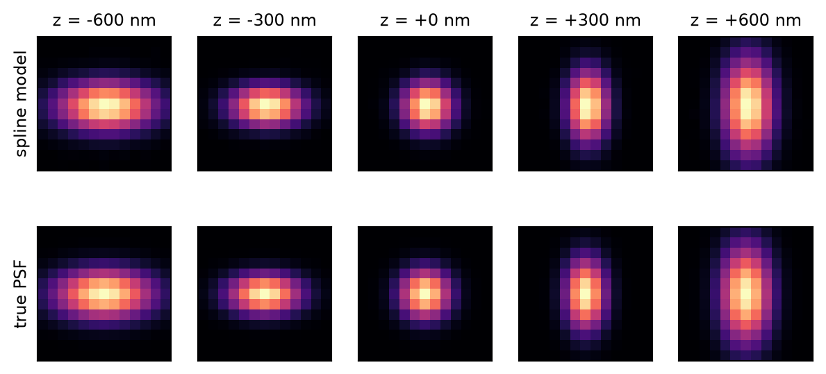
The calibration. Top: the spline model at five heights, as the fitter sees it in a 13-pixel ROI. Bottom: the PSF the simulated beads were drawn with. The spot is stretched along x below focus and along y above it; the model has learnt that from nine beads.

3. The fit. Each ROI is compared with the model: the calibrated PSF at position and height , scaled to photons, on a flat background per pixel. The five parameters that make the observed photons most probable are the result. z is found the same way x and y are: the shape of the spot is what depends on it, and the fit changes z until the model's shape matches the spot's.

The fit starts at the centre of mass of the ROI, at the background of its border pixels, and at the start z – the focal plane of the calibration unless set otherwise. From there Levenberg-Marquardt walks to the best z; with an astigmatic PSF the shape changes monotonically over the range, so there is one best z to find.

4. Precision. As for the Gaussian fitter, the Cramér-Rao lower bound (CRLB) from the model says how precisely each parameter can be known from the photons there are, and it is written as x_err_nm, y_err_nm and z_err_nm. It depends on z: where the spot is small it is sharp and precise; far from focus it spreads over more pixels and more background, and the precision falls. z is typically two to four times less precise than x and y.

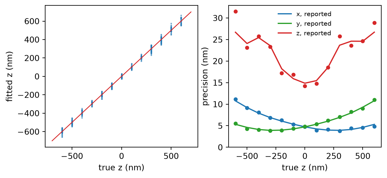
The fit gives z back. Spots simulated at known heights (2000 photons, 10 background photons per pixel) from the true PSF, not from the spline, and fitted with the calibration of the figure above. Left: fitted against true z, with the line of perfect agreement. Right: the scatter of each coordinate about the truth (dots) against the precision the fitter reported (lines) – x and y trade places above and below focus, and z is best near focus.

5. The table. Positions are converted to nanometres with the pixel size (the default units here are nm), fits that failed or whose z is not a number are dropped, and the table is saved as <acquisition>_locs.hdf5.

In detail

The spline. The calibration is a grid of boxes (voxels): one pixel wide laterally, deep. Within each box the PSF is a tricubic polynomial of the fractional offsets of the point from the box's corner, in x, y and z,

so 64 coefficients per box, stored as an array of shape in the order . The Bead calibration tool computes them by not-a-knot cubic interpolation of the averaged bead stack along each axis in turn, after normalising it so that the brightest plane sums to 1 over the calibration ROI; is then the photons in that plane. A SMAP file brings its own coefficients.

The model. For pixel of a ROI centred on the candidate,

where the ROI sits in the middle of the (larger) calibration grid. Its derivatives are those of the polynomial,

and the same for y; z is fitted in units of grid planes and converted at the end. The likelihood, the Levenberg-Marquardt steps (with the expected information as curvature) and the CRLB are exactly those of the Gaussian fitter, with these five derivatives: the Fisher information

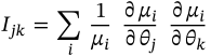
at the fitted , and . Because the model is the measured PSF, the CRLB includes everything the PSF does with z – which is what makes the z precision curve of the figure above come out of the fit rather than from a formula. A calibration made from few, noisy beads has bumps of its own that the fitter takes for information, and then reports a z precision that is too good; smoothing the calibration along z (the Bead calibration's setting) is what prevents it.

z. The spline's z index is converted with the calibration's plane spacing and its focal plane (z0 in the file),

The minus sign is the convention SMAP uses: the calibration records where the objective was, and a bead is below the focus by as much as the objective was raised. z is therefore relative to the calibration's focal plane, not to the coverslip, and in the nanometres the objective moved – no correction for the different refractive index of the sample is made (for an oil objective imaging into water, real distances are shorter, by a factor of roughly 0.7 to 0.8; Math Parser can apply one).

The start and the limits. x and y start at the ROI's centre of mass, the background at the mean of the ROI's border pixels, the photons at the brightest pixel above background divided by the model's central value, times 4, and z at start z (0 nm by default, the plane ). A z step is capped at a third of the calibration's depth (at least two planes) at first, and the cap is halved whenever the step reverses. z is held inside the calibration: a fit that tries to leave it stops at an end. During the fit and ; x and y are not held.

Mirroring. A SMAP calibration made from mirrored bead images (emmirror, for beads read out through the other port of an EMCCD) records that; each ROI is then flipped in x before it is fitted and the fitted x flipped back, so the table is in the orientation of the data. Calibrations from the Bead calibration tool are never mirrored.

EM gain. A calibration records whether the beads were taken with EM gain – the Bead calibration tool reads it from the bead files' metadata, a SMAP calibration carries it – and if the data's camera says otherwise, the fit warns, in the plugin's output: the EM register of many EMCCDs reads out mirrored, so a model from beads on the other port is mirrored against the data, and every fit is then subtly wrong. The fit is not stopped. The EM gain's excess noise is handled as in the Gaussian fitter. So is the camera's read noise: its variance is added to data and model, one electron without EM gain by default (read noise), which also keeps a pixel whose spline model nears zero from dominating a fit at low background (see Gaussian 2D).

Compared with the paper. The method is that of Li et al. 2018; what the code does differently (the first two concern the Bead calibration tool; a SMAP calibration brings its own coefficients):

• The beads' background and scale. The paper subtracts each bead stack's minimum and divides by the summed intensity of its central plane; here each stack loses the median of its border pixels over all planes, and the average is scaled so that its brightest plane sums to 1.
• Smoothing. The paper smooths along z with a smoothing B-spline; here with a Gaussian of smoothing z (20 nm by default), after which negative values are set to zero.
• The fit. The expected information as curvature (see Gaussian 2D); one z start, where the paper fits twice, from 500 nm above and below focus, and keeps the more likely; one read-noise variance for the chip, where the paper's sCMOS model has one per pixel; and no refractive-index factor (the paper multiplies z by 0.75).

Parameters

Output

The table has the columns of Gaussian 2D with z instead of the PSF width:

column	meaning
x_nm, y_nm	the position
z_nm	height relative to the calibration's focal plane, in objective nanometres
z_err_nm	its precision (CRLB)
x_err_nm, y_err_nm, xy_err_nm	the lateral precision (CRLB)
photons, background, photons_err, background_err	, and their CRLB
logl, logl_rel	the log-likelihood, and per pixel
peak_x_pix, peak_y_pix, iterations	the candidate, and the steps taken

The file also records the calibration used: its path, , , the grid and whether it was mirrored.

What to check:

• The z histogram should cover the depth of the sample, with no pile-up at the two ends of the calibration's range – those are fits that ran out of it, and should be filtered away.
• logl_rel separates good fits from bad. Two emitters close together are fitted as one rounder spot, whose z is pulled towards focus; those fits have a poorer logl_rel, and filtering on it is the remedy. In simulations that was the whole of an apparent z compression of 7 %.
• z_err_nm of 10 to 30 nm for a few thousand photons is usual (the figure above); much larger values belong to dim or strongly defocused spots.

The camera frames. The file also keeps a few of the frames the table was fitted from, in photons (counts minus offset, times the conversion): first the average of every frame fitted, then the first fitted frame, then the rest spaced evenly up to the last one, as many as raw frames asks for, each with its frame number – the same number as in frame. In the Render tab they are a source of an image layer, placed in the table's coordinates, so they lie under the localizations: whether a structure is really there, where the cell edge is, or whether the focus was lost can be checked without the original stack. The average is the one to start with; a localization of frame 17 should sit on a spot in frame 17.

Differences from SMAP

Based on SMAP's fit_fastsimple workflow and its MLE_GPU_Yiming fitter in Spline mode (Ries 2020). The main changes:

• The steps, as in the Gaussian fitter: the expected information as curvature and the background started at the ROI's border (together they stop fits at low background from sticking at no background, which in the spline fitter froze z at its start), and no clamp of x and y.
• One z start, at the focal plane unless start z says otherwise. SMAP starts at the centre of the spline grid plus an offset set in the GUI, and accepts several starts, keeping the fit with the best likelihood.
• No refractive-index correction. SMAP's fitter has an optional factor (0.8 by default when switched on); here z stays in objective nanometres.
• Calibrations of its own. The Bead calibration tool follows SMAP's calibrate3D_g, but uses a linear rather than circular correlation to align beads, and crops z to where all accepted beads overlap, which can make its z range narrower than SMAP's.
• Raw frames by number, not by spacing. SMAP's CameraConverter keeps every diffrawframes-th frame after the average; here a number of frames is kept, spaced evenly over the fitted range, so that a long acquisition does not fill the file with them.

References

• Li Y, Mund M, Hoess P, et al. Real-time 3D single-molecule localization using experimental point spread functions. Nat Methods 15, 367 (2018). doi:10.1038/nmeth.4661 – the method: bead calibration, cubic spline model, and the fitter this one follows.
• Babcock HP, Zhuang X. Analyzing single molecule localization microscopy data using cubic splines. Sci Rep 7, 552 (2017). doi:10.1038/s41598-017-00622-w – cubic splines as a model of a measured PSF.
• Huang B, Wang W, Bates M, Zhuang X. Three-dimensional super-resolution imaging by stochastic optical reconstruction microscopy. Science 319, 810 (2008). doi:10.1126/science.1153529 – z from astigmatism.
• Smith CS, Joseph N, Rieger B, Lidke KA. Fast, single-molecule localization that achieves theoretically minimum uncertainty. Nat Methods 7, 373 (2010). doi:10.1038/nmeth.1449 – the maximum likelihood fit and its CRLB.
• Ries J. SMAP: a modular super-resolution microscopy analysis platform for SMLM data. Nat Methods 17, 870 (2020). doi:10.1038/s41592-020-0938-1