Panels
The layers of the picture – which localizations each one shows, and how it is drawn.
A localization table is a list of positions, not an image. To see the structure, every localization is drawn as a small spot on a fine grid and the spots are added up: where many molecules were found, the picture is bright. The Render tab decides what goes into that picture and how it is drawn.
The picture is made of layers. Each layer shows the localizations its own filter keeps, drawn its own way – one layer per channel or per file, say, or the same data twice with different filters. The visible layers are added up into the image in the main window, as in SMAP. Every control below the layer strip edits one layer, the one selected in the strip.
What a layer shows is also what the rest of the program works on. A plugin measures the localizations the layer's filter keeps (inside the drawn ROI, if there is one), and the ROI manager takes its filter and its grouping from a layer too. So a filter set here to clean up the picture also decides what is measured.
From top to bottom the tab has: a small overview of the whole field, the layer strip, the filter, the image section (only for a layer that is a pixel image), the display – how the localizations are drawn – and, closed by default, the axes, which turn the picture into a plot of any column against any other.
1. Layers. A file opens as one layer. + adds another, which starts as a copy of the selected one – a second layer is nearly always the first with one thing changed. A layer can also be a pixel image, placed under the localizations by its pixel size and position: the camera frames the fit kept with the file (their average, and a few single frames), or a widefield or diffraction-limited picture of the same cells. The layers are drawn one by one and their colours added.
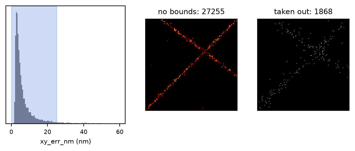
2. The filter. A filter is a range per column: keep the localizations whose precision is at most 25 nm, whose z lies within 500 nm of focus, and so on. A localization is shown only if it is inside every range. The tab shows one column at a time, as a histogram with the kept range shaded, and the range can be dragged or typed. A new layer opens with a few bounds already set (see In detail), so that fits which are clearly bad are left out from the start – and are left out visibly, in the shaded histogram, rather than silently.
A simulated ring-and-cross structure. Left: the localization precision of all localizations, with the range the default bound keeps shaded. Middle: every localization. Right: what the default bounds take out – mostly the dim, imprecise localizations scattered around the lines.
3. Grouping. A fluorophore that stays on for several camera frames is localized in each of them, so one blink appears as a small cluster of localizations. Grouping links the localizations of consecutive frames that lie within a small box of each other into one blink and replaces them by a single localization – at their weighted mean position, with the photons of all of them and a correspondingly better precision. A grouped picture is cleaner and counts molecules more fairly: a long blink no longer weighs more than a short one. Layers are grouped by default (grouped); the linking distance and the number of dark frames allowed are set under link settings..., beside it, for every layer at once.
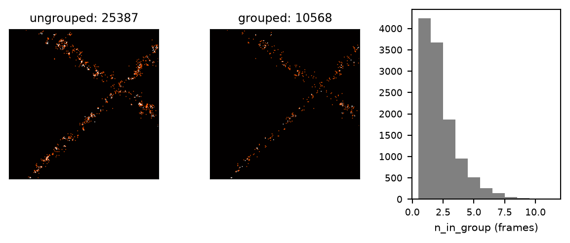
The same localizations (with the default bounds, drawn as a histogram) before and after grouping, and how many frames each blink was linked over.
4. Drawing the localizations. render chooses the spot each localization is drawn as. hist counts localizations per pixel: exact, but at a fine pixel size mostly single bright pixels. gauss draws every localization as the same Gaussian blob, of width sigma x (gauss). precision, the default, draws each one as a Gaussian as wide as its own localization precision times the precision factor (Baddeley et al. 2010): a precise localization is a sharp dot, an uncertain one a faint wide blur, so the picture shows how well each position is known. dl (diffraction limited) draws what the camera saw instead: each localization as a spot as wide as its fitted PSF, on the camera's own pixels – the widefield picture of the same molecules, to set beside the super-resolved one.
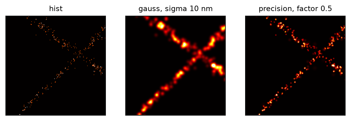
The crossing of the two lines, 800 nm across, drawn with each of the three super-resolution modes.
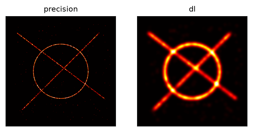
The whole field, 10 µm across, in precision and in dl: on 100 nm camera pixels the ring and the lines are as wide as the PSF, as the camera saw them.
5. Brightness and colour. A super-resolution image has a few very bright pixels – a long blink, a fiducial bead – and a great many faint ones, so its brightest pixel is a useless scale. contrast instead saturates a fixed fraction of the pixels: at contrast 3 the brightest one in a thousand are white, at 2 one in a hundred (brighter), at 4 one in ten thousand (darker). gamma below 1 lifts the faint parts further. The LUT (look-up table) is the colour scale brightness is shown in. Instead of brightness alone, the colour can also encode a column (colour by, e.g. z), with the brightness still showing density.
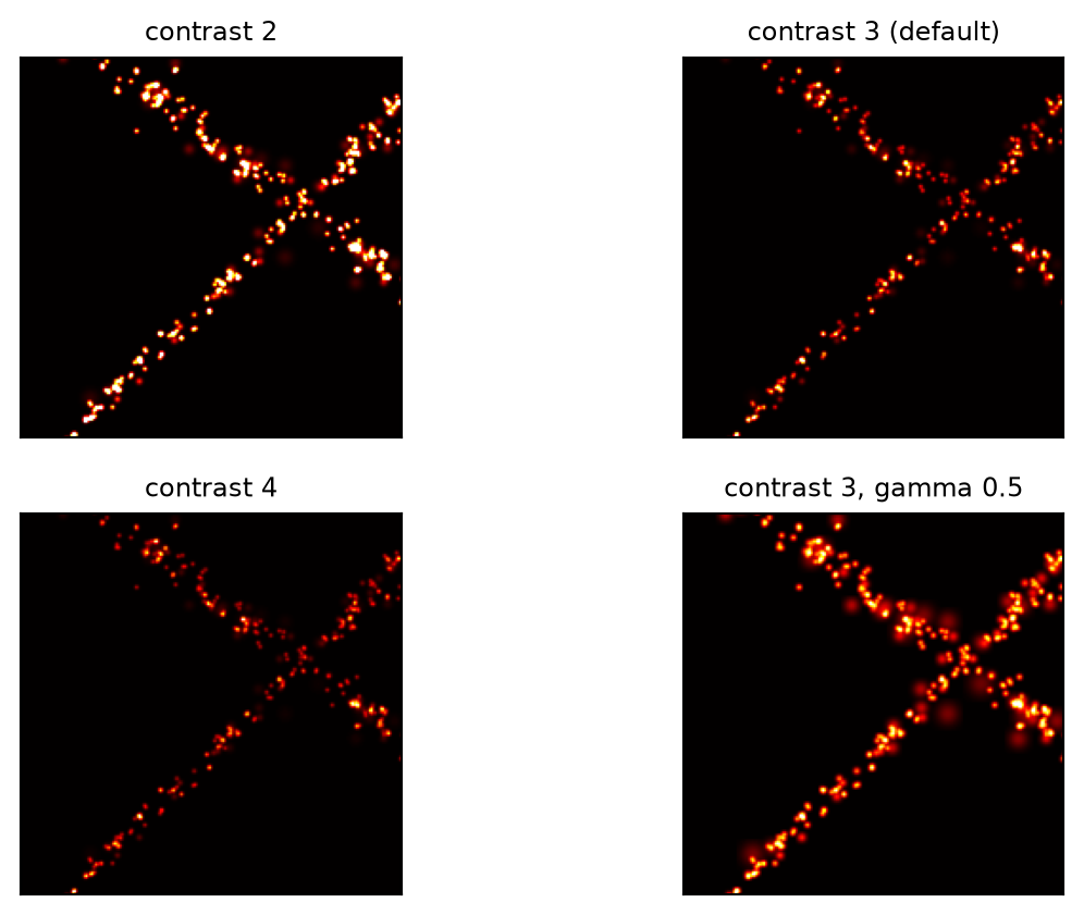
The same crossing at three contrasts, and with gamma 0.5.
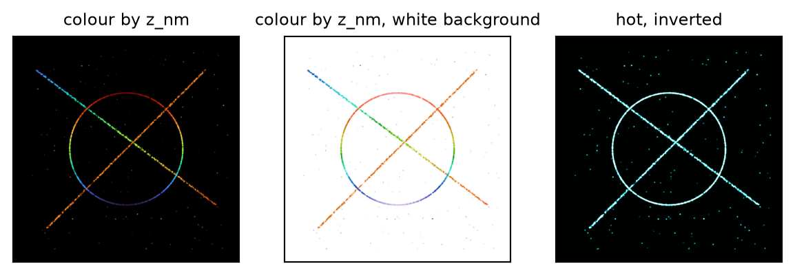
The whole field coloured by z: the ring is tilted, so its top and bottom lie at different depths, and the two lines are at slightly different heights. The same on a white background, and the plain picture with the LUT inverted.
6. Any column against any other. The axes section says which column each axis of the picture is. Normally that is x and y, and the picture is a picture of the sample. Choose z for the vertical axis and it is a side view; choose frame and photons and it is a plot of brightness over the acquisition – drawn with the same layers, filters, colours and ROIs as the image. This is how bleaching, a change of laser power or a drop in quality over time is seen at a glance.
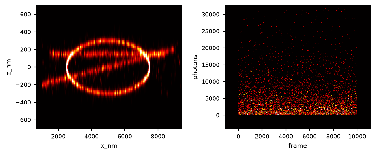
Left: z against x – a side view of the tilted ring and the two lines (z stretched for the figure). Right: photons against frame, one dot per blink.
The rendering kernel. Each localization contributes the integral of its Gaussian over each pixel, not the Gaussian's value at the pixel centre:

with  ,
,  the pixel edges. The kernel is cut off at 2.7
  and normalised by its own sum over the pixels it reaches, so every localization adds exactly one to the image, whatever its width and wherever it sits in its pixel; a histogram is the limit
  of the same kernel. A pixel
  covers
  for pixel size
  .
.
The width in precision mode. With  the localization precision of localization
  (
(xy_err_nm),  the precision factor (0.5 by default) and
  the rendered pixel size,

The floor of 0.7 pixels keeps a very precise localization from vanishing between pixels; it follows the zoom, since the main view renders at the screen's resolution. The cap keeps a handful of absurd precisions from smearing over the picture and from dominating the render time. A missing precision is drawn at the floor. On an axis that is z, the axial precision z_err_nm is used where the fit produced one. On an axis that is not a position at all (photons, frame), there is no precision, and the explicit width is used – zero, plain binning, unless set.
The dl mode. As SMAP's DL: the picture is rendered on a grid of camera pixels – their edges on multiples of the pixel size  , which comes from the fit's metadata (
pixelsize_nm, or the camera's), a simulation's optics, or 100 nm – with each localization a Gaussian of width sigma_nm (and sigma_y_nm vertically, where the fit had two), and then blown up to the view pixel by pixel, without interpolation, so that the camera's pixels stay visible. A width that is missing, not positive or above 1500 nm (a failed fit) is one camera pixel. It needs the positions on both axes; the 3D view, whose turned picture no camera saw, draws it as gauss at the median PSF width.
Contrast and gamma. With  the rendered intensity of a pixel and
  the contrast, the pixel value that becomes full scale is the quantile

that is,  of the pixels are saturated (if that quantile is zero, as in a very sparse image, the maximum is used). The displayed value is
  with
with  the gamma, and
  picks one of the LUT's 256 colours. Contrast and gamma change only this last step, so moving them does not render again.
Colour by a column. Each localization gets the LUT colour of its value  in the colour range
  (values outside take the end colours). Colours are added up during rendering, together with the plain count; the displayed hue is the average colour of the pixel and its brightness the count, put through contrast and gamma as above. A dense pixel therefore keeps its hue instead of bleaching to white. Choosing a column starts its range at its 0.5th to 99.5th percentile and switches the LUT to turbo; going back to intensity switches it to hot. Because the colour is part of the rendering here, changing the LUT of a coloured layer renders it again.
Inverting, and the white background. With  a LUT colour, invert's SMAP choice gives
  per channel (SMAP's
 lutinvert), and its grey choice gives  , the opposite hue at the same lightness, so that a layer over its inverse turns grey where they coincide. white background turns the brightness over and keeps the hue,
  : black becomes white, a saturated red stays red. It is applied once, to the sum of the layers.
Adding up layers. The RGB images of the visible layers are added and clipped at 1. Two layers in red and green therefore show yellow where both are bright.
The filter. A bound  on a column keeps
  ; an empty end is no bound. A localization with no value there (NaN) is excluded by any bound on that column – a localization without a z is not in a z slab. The shown set is the intersection of all bounds and of the file choice. A new layer starts with
 xy_err_nm at most 25 nm, logl_rel at least -2 and z_nm between -500 and 500 nm, plus sigma_nm at most 180 nm on a 2D table (in 3D the PSF width changes with z by design), each only if the table has that column, and any bounds the file carries from Remove Localizations. A bound applies to the grouped and the ungrouped table alike, so what is drawn and what a plugin gets never disagree. The histogram spans the bulk of the column in 120 bins (of a random sample of two million, for a larger table): the 1st to 99th percentile, cut to three interquartile ranges beyond the quartiles, so that the long tail of a precision column – a few faint spots with errors of hundreds of nanometres – does not squeeze the rest into one bar. As in SMAP, dragging an edge of the shaded range to the end of the histogram removes that end of the bound, so the tail is not cut off, and anywhere else it is the number. Only the dragged end changes: a bound that lies beyond the histogram (the 25 nm one, on a sharp table) stays until its own edge is moved or its number typed.
Grouping. The linking follows SMAP's: the localizations are sorted by frame and x, and each one not yet linked starts a new blink. From the blink's running position it looks in the next frame for the first unlinked localization inside a box of half-width  (link within, 50 nm) in both x and y – the first found, not the nearest – and moves the running position halfway towards it. A blink may skip up to gap dark frames (1) before it is closed. Files and channels are linked separately. Each blink then becomes one row: positions weighted by
  (x by
(x by x_err_nm, y by y_err_nm, z by z_err_nm where the table has them), photons and background summed, precisions combined as  , the error of a summed quantity as
  ,
, logl_rel the best, frame the first. n_in_group, the number of frames the blink was on, and group_id are written onto both tables. Grouping is done once per table and kept; switching grouped back and forth costs nothing after the first time.
The axes. A coordinate is the column divided by that axis's scale,  , and the render grid stays square in these units – so the zoom, the ROIs and the 3D box work unchanged, and the two scales are what makes a pixel represent, say, 5 frames across and 20 photons up. Choosing a column (or fit) sets each scale that is not a position to a round 1, 2 or 5 times a power of ten, at or below its 1-99 % span divided by 1000 (or by the span of a position axis shown beside it), and frames the view on that span. A position axis keeps a scale of 1, so that a picture of x against z is still a picture of a place. On any axis that is not a position the rendering width is set to zero (plain binning), and put back on the way back to x and y.
The whole field of view, small, with a yellow frame where the main view is; click in it to move the main view there. It draws itself when a table is opened; it can be taken out into a window of its own.
Draws the overview again with the current layers – after a filter, a LUT or a layer has changed.
Adds a layer: localizations or image.... The layer strip also has one button per layer: click to edit it, right-click to show or hide it without selecting it; bold means drawn, struck through means hidden.
Whether the selected layer is drawn. A hidden layer keeps its settings and is still what a plugin reads when it asks for that layer.
The selected layer's name, shown in its button's tooltip and in the layer lists of the dialogs that ask for one.
A new localization layer on the same table, starting as a copy of the selected one – its bounds, files, display and grouping – and the tab moves onto it.
Adds an image layer. When a file open has camera frames kept with it, the new layer shows their average; otherwise it asks for a TIFF or PNG. If the file does not say its pixel size, a dialog asks for it and for where its first pixel lies.
Removes the selected layer. There is always at least one.
Copies settings from another layer onto the selected one. Only the display is ticked at first: the bounds and the files are usually what makes two layers two.
The quick buttons (prec, LL, frame, z, phot, PSF, ch, file) pick the usual columns; the drop-down has every numeric column. A column with a bound on it is bold and marked with a dot, so a bound on a column not on show is not forgotten. The count reads shown / all, and how many are in the ROI when one is drawn. For filenumber the histogram is replaced by a list of the files to tick; right-click a file to remove it from the session.
The lower bound; empty is none.
The upper bound; empty is none.
Removes the bounds on the column shown.
Ticks every file.
Unticks every file – the layer then shows nothing until one is ticked.
Shown instead of the filter for an image layer: where the image lies under the localizations.
What the layer shows. The list has the camera frames each open file kept (name: raw frames – the average of every fitted frame, then single frames spaced over the acquisition, in photons), every image opened, and open file... for another TIFF or PNG. The kept frames are placed by the camera's pixel size and ROI, so they lie under the localizations without adjusting anything. Saving the localizations keeps the kept frames and every image a layer shows in the file, with their pixel size and position, and opening it again offers them here.
Must be the image's real pixel size in the sample, or it will not line up with the localizations.
Where the image's first pixel lies in x, in the localizations' coordinates. Adjust it (and y0) to register the image to the localizations.
Where the image's first pixel lies in y.
For a stack, which frame is shown; the label beside it says which – average of 2000 frames, or frame 17, the number the frame column uses. Each layer has its own, so two layers can show the average and one frame.
How the selected layer is drawn. An image layer uses only the LUT, contrast, gamma and white background.
precision for the usual picture. gauss when every spot should look alike, e.g. to compare layers of different quality; hist for counting, or at a pixel size well above the precision. dl for the widefield picture: zoomed out it looks like the average of the raw frames, which is a check that the fit found what was there.
intensity colours by brightness through the LUT; field colours by the column chosen beside it.
The values that get the two ends of the LUT. Narrow it to spread the colours over the part of the range that matters – for z, the depth of the structure rather than of the outliers.
Sets the colour range to the column's 0.5th to 99.5th percentile.
Hot for intensity, turbo for a column. For several layers, one pure colour each (red, green, cyan, magenta) adds up legibly.
The opposite colour at the same brightness: red becomes cyan. Beside it, which inversion: SMAP as SMAP does it (inverted hot runs through cyan to white), grey so that a layer over its inverse goes grey where they overlap. For black on white, pick the gray_inverted LUT or white background instead.
3 is a good start. Too low, and the structure saturates into white bands; too high, and all but the brightest spots disappear. The same number transfers between datasets, because it is a fraction of pixels, not a brightness.
Draws one localization per blink. The first switch links the table, which takes seconds to minutes on a large one; after that it is free. Plugins get the ungrouped table unless they ask for the grouped one.
The linking parameters of grouping, link within (nm) and gap (frames), for every layer at once. OK groups all the layers again and records the new parameters in the file's history, since the grouped table cannot tell which ones produced it.
The rendering widths, gamma and the white background.
The width in mode gauss, in the units of the horizontal axis; 0 bins. A few times the pixel size, or about the typical precision.
The vertical width, for axes that are not the same quantity. Empty follows sigma x where the two axes are the same quantity and bins where they are not.
0.5 draws each localization at half its precision: sharper than the statistics strictly allow, which is what makes fine structure readable. 1 is the honest width; much below 0.5 the spots fall apart into single pixels.
Below 1 lifts the faint parts, above 1 suppresses them. 1 keeps the brightness proportional to density.
The picture on white paper, the hue kept: for figures and print. It is set on every layer at once.
Which column each axis of the picture is. Set on all layers at once; closed, it is the ordinary picture. While a custom pair is shown, a note says what is across and up, and the scale bars are in the axes' own units.
The horizontal axis, and after scale how many units of that column one render unit is. auto is the table's x position.
Units of the axis's column per render unit. For positions leave it at 1; for photons against frame, fit picks scales that make each axis's 1-99 % fill the picture.
The vertical axis and its scale. auto is y.
The third axis in the 3D view and its scale. auto is z.
Ticked by itself when the two axes are the same quantity, so that distances stay true; x against z stretched would misrepresent the structure.
Scales each axis so its 1-99 % fills the picture, and frames the view on it. It is done by itself when a column is chosen.
Back to x against y, the ordinary picture.
Based on SMAP's layer panel (gui.GuiChannel), its renderer (renderSMAP, drawerSMAP) and its VersatileRenderer plugin (Ries 2020).
logl_rel from -2 (SMAP -1 to 0) and a PSF bound of 180 nm (SMAP 175) only for 2D data; z within 500 nm is the same.