Panels
A box of the data, the slab, shown from any angle, with the Render tab's layers, filters and colours.
A 3D localization table is a cloud of points in a volume. The usual image of it is the view from the top: z is thrown away, or turned into a colour. Many structures only make sense from the side. The two rings of a nuclear pore lie on top of each other when seen from above, and a microtubule seen from above does not show whether it is hollow.
The 3D view shows a box of the data, the slab, from any angle. You cut out a small volume around what you want to see, with an ROI in the 2D view, and turn it with the mouse. The picture is drawn the same way as the 2D image: the layers, filters, look-up tables and colour fields of the Render tab all apply. Only the direction you look from is new.
The slab can also be the selection for plugins (plugins use the slab (while open)). A measurement then sees only what is inside the box, for example one ring of a pore picked out by its depth.
Use it on tables with a z_nm column. A 2D table can be opened too, but it is flat: from the side it is a line.
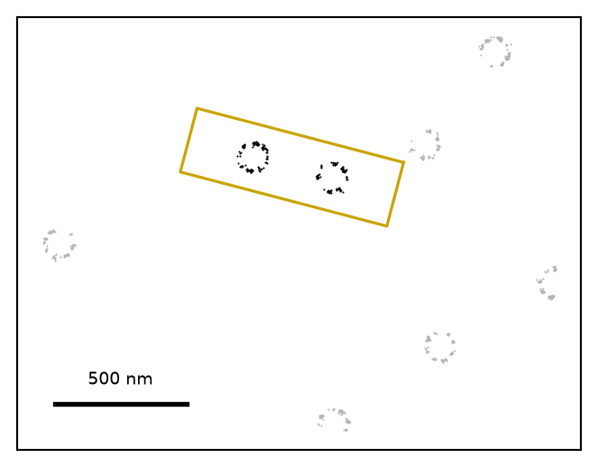
1. The slab. The slab is a box in the data. Its footprint comes from the ROI drawn in the 2D view. A rectangle gives an upright box. A line ROI gives a box turned in the plane: its length is the line, its width the line's width, and its angle the line's direction. Any other ROI gives its bounding rectangle, and no ROI the whole field. The depth of the box is the z range the layer's filter lets through, or all of the data's z if there is no z filter. While follow 2D ROI is ticked, the box follows the ROI as it is drawn or dragged.
Simulated nuclear pores (Nup96) seen from the top. A line ROI drawn through two neighbouring pores becomes a slab turned in the plane (yellow): its long axis is the line, its width the line's width. The localizations inside it (black) are all the 3D view draws.
2. Turning it. Only what is inside the slab is drawn. Each of those localizations is turned by a rotation  into view coordinates: two across the screen, and a third, the depth, pointing at the viewer. Dragging with the mouse changes
  . The buttons top, front and side look at the slab from above, along its width and along its length. The box's edges are drawn over the image, and a small tripod in the corner shows where the slab's own x (red), y (green) and z (blue) point.
3. Drawing it. The turned localizations are rendered with the 2D renderer, each layer with its own settings, as if the turned slab were a flat table. Everything between the front and the back of the box adds up on the screen. Optionally the far side is dimmed (dim with depth), the front hides the back (opacity), or the colour says how near each localization is (colour by depth).
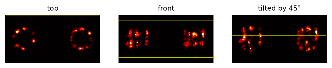
The slab above, from the top, from the front (along its width, so z is vertical) and tilted by 45°. From the top each pore is a ring; from the front the two rings of each pore, 50 nm apart in z, are seen edge on.
4. While the mouse moves. A drag draws a quick preview: at half the resolution, and from a sample of the localizations sized so that the picture keeps up with the mouse on the machine it runs on. When the mouse stops, the full image is drawn from every localization in the slab. An image that is saved is always the full one.
5. The slab as the selection. With plugins use the slab (while open) ticked, every plugin's selection is cut to the slab, on top of the layer's filter and the 2D ROI. This holds only while the 3D window is open, so that nobody measures a box they can no longer see.
What is inside the slab. The slab has a centre  , a size
  and an angle
  in the plane. For a localization at
  , its position in the slab's own frame is

and it is inside when  ,
,  and
and  . The edges count as inside. A table without z is taken to lie in the slab's centre plane, so only the footprint decides. The box is tilted only about z: its top and bottom are always planes of constant z.
The rotation. With  a data point and
  the centre of rotation (the pivot), the view coordinates are

with  the azimuth (a turn about the data's z axis),
  the elevation (a tilt about the screen's x axis; 0 is the view from the top) and
  the roll (a turn about the line of sight).
  and
and  are the screen,
  the depth, positive towards the viewer. The presets set
  to
to  for top,
  for front and
  for side, with the slab's angle subtracted from
  so that they are views of the slab and not of the data's axes.
With fix roll ticked (the default) a horizontal drag changes the azimuth, a vertical one the elevation, and the roll stays zero, so the horizon stays level. Unticked, the drag turns about the screen's own axes, like a trackball. The mouse turns 0.4° per pixel, and the arrow keys 5° per press. With rotate about the screen centre ticked, a turn is about the point in the middle of the screen rather than the slab's centre, so that after a pan the view does not swing away from what is being looked at.
Perspective. Off, the projection is orthographic: parallel edges stay parallel. On, with  the eye's distance, the screen coordinates are scaled by

so that what is nearer is larger. The distance starts at ten times the slab's longest side and follows the slab until it is typed in.
Depth. The depth range is that of the slab's eight corners, not of the localizations, so that colours and dimming do not change with the filter. Dim with depth weights each localization by  ,
,  the length set, so that the front face is at full weight. Opacity
  cuts the depth range into slices slabs and draws them from the back to the front: with
  the image of slice
  and
and  the brightness the plain image is shown at, each slice covers what is behind it by
  ,
,

At  this is the plain sum. The same compositing is done for the colour.
The preview. While dragging, the grid is two times coarser and at most about 13 localizations per pixel are drawn, fewer if the last frames took longer than 1/27 s. The sample is evenly spaced through the table, which is in acquisition order, so it is a shorter acquisition rather than a rearranged one.
The depth histogram. Under the controls is a histogram, in 64 bins, of the depths of up to 200 000 of the slab's localizations, over all visible layers. It shows where along the line of sight the data are, for placing the slab.
Other axes. When the Render tab draws one column against another (its axes section), the slab is a box in those units and is rebuilt over the whole field when the axes change. The scale bar is then hidden, and each arm of the tripod is labelled with its own column and a round length in its units.
The window has the image and a toolbar; the controls are a window of their own beside it (controls).
In the image: drag to turn, shift-drag (or the middle button) to pan, the wheel to zoom. Alt-wheel or page up / page down moves the eye and the centre of rotation along the line of sight. Ctrl-wheel moves the slab along the line of sight by a tenth of its smallest side per step; shift-wheel makes it thicker or thinner along the axis nearest the line of sight. The dots on the box are its faces: drag one to move that face. Moving a face, like typing a range, stops the slab from following the ROI.
PNG as displayed... saves the picture as it is on screen. The two TIFF entries ask for a pixel size and render the slab again, at full resolution, to fit the box exactly: in colour, or as the summed intensity in floating point for measuring. The TIFF records the projection and the slab.
The slab from above. Also in the controls window.
The slab along its width: its length across the screen, z vertical.
The slab along its length: its width across the screen, z vertical.
Centres the slab and zooms so that it fills the window.
Shows or hides the controls window. Closing that window unticks it.
The slab takes its footprint from the 2D ROI every time the ROI changes. Editing the ranges or dragging a face unticks it.
Takes the footprint from the ROI once, and the depth from the z filter, now.
The slab's extent along its own first axis, in nm; for a slab turned by angle, that is along the line, not along the data's x. The y and z rows are the other two axes. Changing one side leaves the other where it is.
The slab's turn in the plane. A line ROI sets it to the line's direction.
Keeps the data's z axis in the vertical plane of the screen, which is the easy way to keep one's bearings. Untick for free rotation.
Off, the slab's centre is always the centre of rotation, which is right as long as the slab is in view.
The attenuation length  ; 0 is off. A value around the slab's thickness along the line of sight makes the front stand out without losing the back.
0 is a plain sum and fastest. Values of 0.3 to 0.7 give a sense of what is in front; 1 hides everything behind a bright slice.
How many depth slices opacity composites. More give a smoother result and cost proportionally more time.
Tick for a perspective view; the number is the eye's distance in µm. Nearer exaggerates depth; much farther is nearly orthographic.
Colours every layer by the depth in the current view, over the depth range of the slab's corners, in place of the layer's own colour field.
CPU and GPU draw the same image; GPU is faster on large tables. GPU points draws each localization as a small round sprite with transparency, and GPU spheres as a shaded sphere with ambient occlusion. Without a usable GPU the CPU is used, and the label under the menu says so. The controls an engine does not use are greyed out.
For GPU points and GPU spheres: the radius in nm. 0 uses the median localization precision of what is shown.
For GPU points: how opaque one sprite is. Many sprites pile up on one pixel, so a useful value is small (the default 0.05).
For GPU spheres: how strongly spheres shade their neighbours; 0 is off.
For GPU spheres: how far the shading reaches. 0 takes three sphere radii, or a twentieth of the slab's smallest side if that is larger.
Draws the slab's edges and the face handles. The handles are needed to drag a face.
The scale bar is a length in the plane of the screen. The tripod shows the slab's own axes, projected like the data, so an axis pointing at the viewer is short.
Off by default. On, the selection name every plugin reports ends with the slab's size, so the history says that a box was used. Closing the window lifts the restriction; opening it again restores it.
Based on SMAP's sr3D/Viewer3DV01 (Ries 2020).