Localization Statistics

Analysis › Measure · version 3

Photons, localization precision and on-time, each with its law fitted.

What it does

Three histograms that say whether a dataset behaves as SMLM data should, and how good it is:

photons per localization – how bright the fluorophores are;
localization precision – how well each position is known, laterally and, for 3D data, in z;
on-time – for how many consecutive frames a fluorophore stays on.

Each has the law it is expected to follow fitted over it, so a glance says whether the data look normal, and the fitted numbers are what to compare between samples, dyes, buffers or days: the mean photon count , the typical precision and the mean on-time .

It describes the localizations of the layer as they are shown – after its filter and inside the ROI – unless localizations is set to all.

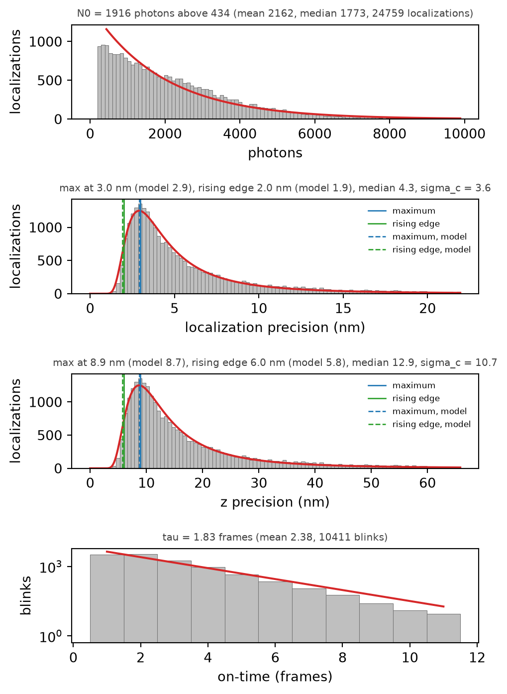
What the plugin shows, here for a simulated dataset filtered at 200 photons: photons, lateral and axial precision, and on-time. Grey: the histogram. Red: the fitted law. Blue and green: the maximum and the rising edge of the precision, solid as read off the histogram, dashed where the fitted model puts them.

How it works

Photons

A fluorophore that is switched on emits until it switches off or bleaches. If it does so at a constant rate, the number of photons collected in one localization is exponentially distributed,

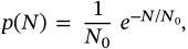
and the single number – the mean photon count – describes it. A larger means brighter localizations and better precision.

The histogram is exponential only above its maximum. Below it the detection threshold has removed the dim localizations, so the fit starts at the maximum (or at photons from, if that is set). The fit is maximum likelihood on the localizations above the start, which for an exponential is simply

the mean of what is left above the start, minus the start. It does not depend on the bins of the histogram.

Localization precision

The precision of a fit is set by the photons: to a good approximation

with a constant of the PSF, the pixel size and the background. If is exponential, has a distribution of its own, which follows in two lines: exactly when , so

One parameter again, and it has a meaning: is the precision at the mean photon count . The curve rises steeply from zero, peaks, and has a long tail of poorly localized, dim molecules:

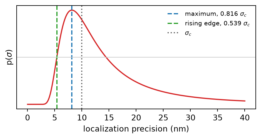
The distribution of the precision that exponential photons imply, for = 10 nm, with its two landmarks. The rising edge is where the curve first reaches half its maximum.

Two positions on the curve follow in closed form, and both can be read off a histogram by eye:

the maximum, at ;
the rising edge, where the curve first reaches half its maximum, at .

The rising edge is the precision of the best localizations, the ones that decide the finest detail an image can show.

The plugin reports both twice: fitted (the model's landmarks, dashed) and read off the histogram itself (solid). They agree when the photons really are exponential, and part company when they are not – when the fitter returned a population of failed fits, say, or when the sample mixes two dyes. That comparison is the point of printing them side by side.

The precision is fitted to its histogram by least squares, not by maximum likelihood on the localizations, because it is robust that way: a fitter always returns a few rows with an absurdly small precision, a fraction of a nanometre, which are failed fits and not good localizations. The likelihood weighs each localization by , so a few per cent of those rows carry the answer and pull down by an order of magnitude. Binned, they are a few counts in the first bins and move nothing. Precision fit switches to the likelihood for anyone who wants it.

The z precision, when the table has one, is described the same way.

On-time

How many consecutive frames a fluorophore stays on before it blinks off, one number per blink, from the linking of localizations into blinks. If it switches off with the same probability in every frame, the on-time (in frames) is geometric,

which is a straight line on the logarithmic axis the plugin draws it on. The maximum likelihood estimate is the mean, , and the plugin reports the equivalent exponential lifetime

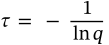
in frames, and in milliseconds if the exposure is given. is what the curve decays with, which makes it comparable to a switching or bleaching time measured some other way.

The on-time needs the localizations linked into blinks: switch the layer to grouped once, and the plugin reads the result. It does not link by itself, because linking can take minutes on a large dataset; it says so instead.

In detail

Which table. The one the layer shows. A grouped layer is described blink by blink – the photons of a blink added up, the precision that of the combined position – and an ungrouped one frame by frame. The on-time is the exception, because it is a property of a blink: it is counted once per blink whichever table is shown. (Counting it per frame would count a three-frame blink three times and a one-frame blink once, and weigh the histogram towards long blinks.)

The photon histogram is drawn up to the 99.9th percentile; the fit uses every localization above the start.

The precision fit. The histogram runs from zero to the 99.5th percentile of the precision, in bins bins, and the model is integrated exactly over each bin (the density changes too fast near zero to be sampled at the bin centre). Its amplitude is solved for directly, so the fit searches one number, : over a wide logarithmic grid first, then by golden section on the best bracket. The unbinned likelihood alternative uses that is exponential with mean – it is – and fits it as the photons are fitted, truncated where the sample was cut.

The landmarks read off the histogram. The counts are smoothed by a Gaussian of one bin, the maximum is refined with a parabola through its neighbours, and the rising edge is the last crossing of half the maximum before the peak, interpolated between bins.

Too few. Below 20 values a distribution is shown without a fit.

Parameters

setting	default	what it does
localizations `source`	as plotted (filter and ROI)	The localizations on screen, or the whole table. Choices: as plotted (filter and ROI); all, unfiltered
bins `bins`	100	The photon and on-time fits are on the localizations and ignore this; the precision fit is on these bins. Only the precision fit and the pictures depend on it. at least 5
precision fit (more) `precision_fit`	least squares on the histogram	The likelihood weighs a localization by 1/sigma^2, so a few failed fits with a precision near zero carry the answer; the binned fit does not see them. See How it works: the histogram fit is robust to the failed fits every dataset contains; the likelihood is the efficient estimator on clean data. Choices: least squares on the histogram; maximum likelihood (outlier-sensitive)
photons from `photon_start`	0 photons	Where the exponential fit starts; 0: at the maximum of the histogram, below which the detection threshold has eaten the dim localizations. Setting it higher than the maximum of the histogram fits only the bright tail, which is useful when the dim end is distorted by more than the threshold – a second, dim population, for example.
exposure (more) `exposure_ms`	0 ms	0: the on-time is reported in frames only.

Output

Plot: one panel per distribution, as in the figure above.
Text: the numbers, one line per distribution: and the mean and median photons; the maximum and rising edge of the precision, from the histogram and from the model, its median and ; and the mean on-time. If the on-time could not be shown, the reason.

What to expect: of a few thousand photons for a good organic dye in a good buffer, fewer for fluorescent proteins; a lateral of about 10 nm or better; an on-time of one to a few frames. A precision histogram whose landmarks disagree strongly with the model's is worth a second look at the fit or the filter.

Differences from SMAP

Based on SMAP's Analyze/measure/Locstatistics (Ries 2020), which shows the same histograms and reports the same numbers. What changed:

Photons. SMAP fits an exponential to the histogram by least squares, from 1.2 times the position of its maximum. Here it is maximum likelihood on the localizations from the maximum on, which does not depend on the bins.
Precision. SMAP reads the maximum and the rising edge off the histogram and draws a log-normal over it as a guide. Here the same two landmarks are read off the histogram, and the model that exponential photons imply is fitted as well, so the two can be compared.
On-time. SMAP fits an exponential to the histogram of the on-time. Here the geometric law is fitted by its mean, and each blink is counted once, whichever table the layer shows.

References

Mortensen KI, Churchman LS, Spudich JA, Flyvbjerg H. Optimized localization analysis for single-molecule tracking and super-resolution microscopy. Nat Methods 7, 377 (2010). doi:10.1038/nmeth.1447 – the precision of a fit and its scaling.
Thompson RE, Larson DR, Webb WW. Precise nanometer localization analysis for individual fluorescent probes. Biophys J 82, 2775 (2002). doi:10.1016/S0006-3495(02)75618-X
Ries J. SMAP: a modular super-resolution microscopy analysis platform for SMLM data. Nat Methods 17, 870 (2020). doi:10.1038/s41592-020-0938-1