Blinking Structure

File › Simulate · version 4

A labelled structure, blinking: localizations to try, or camera frames

What it does

To test an analysis you need data where the answer is known. This plugin makes such data. It takes a structure – a ring, filaments, nuclear pores – puts fluorophores on it, lets them blink the way a dye does, and gives either the localizations a fit would have produced or the raw camera frames for a fitter to fit.

Both outputs come from the same molecules. With the same settings and seed, the localizations and the frames describe the same fluorophores blinking in the same frames. So you can look at a simulation as localizations first, and then fit it from its frames by changing only simulate.

Use it to:

• try the analysis plugins without a microscope (the tutorials do);
• see what a labelling efficiency, a linkage error or a dye's blinking does to a picture or a measurement;
• test a fitter, a filter or a drift correction against the truth, with Ground Truth.

It is a model, not a microscope. The background is flat, the spot is a Gaussian (or a measured PSF), and the dye has one on-state and one off-state. What it tests is whether an analysis gets back what was put in.

How it works

1. The structure. A structure is a file that says where the labels are, in nanometres. It is written in YAML, a plain-text format, as a list of elements: single points (or a table of them), lines, circles, filled polygons, or a grey-scale image whose brightness sets the density. Points are placed exactly where the file says. The other elements are filled at a density (labels per nm of line, or per nm² of area), with the number of labels drawn at random around that density, so no two simulations are alike. A structure can be repeated as copies over the field of view, placed at random or on a grid, turned, tilted and jittered.

The built-in structures are the files in smappy/data/structures, and each one is also an example of the syntax:

• demo – a slightly tilted ring 5 µm across, two crossing lines and a few scattered labels over 10 × 10 µm, in 3D. The ring is dye 1, the rest dye 2. The tutorials measure it.
• npc – nuclear pore complexes labelled at Nup96: 32 labels per pore in two rings 50 nm apart in z, radius 53.7 nm (Thevathasan et al. 2019), two pores per µm², each turned at random.
• filaments – 40 straight filaments, 3 µm long, placed and turned at random.
• pie – a resolution star after ThunderSTORM's (Ovesný et al. 2014): 32 wedges, 4 µm long, alternately labelled and empty. The gap between two spokes narrows towards the centre – a fifth of the radius, so 50 nm at 255 nm from it – and where the spokes merge is the resolution. The labelled wedges rise in density by √2 each, from 25 to 4525 labels per µm², so the same picture shows where localizations start to overlap.

A new structure is a YAML file chosen as the structure file, or dropped into that folder to become a built-in.

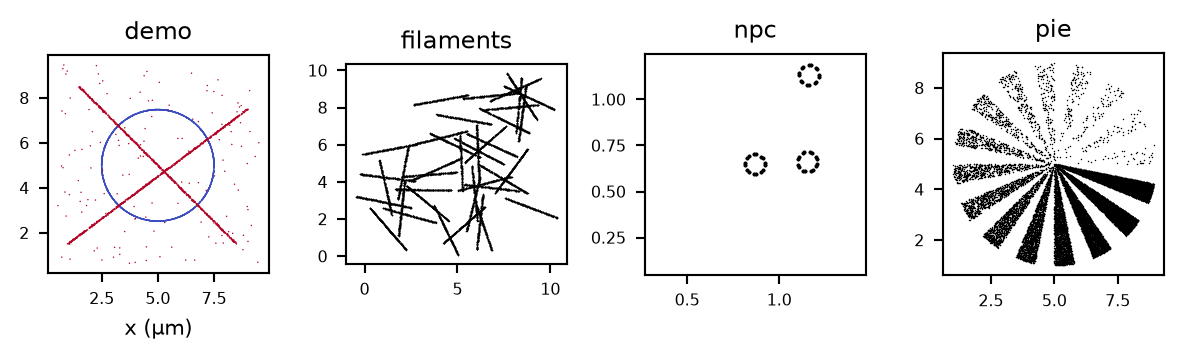
The four built-in structures, as label positions. The pores and filaments are copies of one element, each placed and turned anew; the pie's spokes rise in density going anticlockwise from the right.

2. Labelling. Not every label carries a fluorophore. Each one does with the labelling efficiency, and then carries one fluorophore – or another fixed number, or a random (Poisson) number around it. A fluorophore does not sit exactly on its label: an antibody or a linker holds it a few nanometres away. This linkage error comes in two kinds. A fixed one moves the fluorophore once, and all its blinks share the offset. A free one is drawn anew for every blink, as for a dye that turns on a flexible linker.

3. Blinking. Each fluorophore switches between a dark state and a bright state. It stays dark for a random time (on average the off time) and bright for a random time (on average the on time), and after each blink it bleaches for good with the bleaching probability. The same model serves STORM, PALM and PAINT; PAINT is a long off time. Switching happens at any moment, not only at frame boundaries, so the first and last frames of a blink are dimmer than the ones in between.

Nobody knows the off time of a dye, but one knows roughly how often a molecule comes back in an experiment. So the plugin asks for blinks, the mean number of blinks per fluorophore within the measurement, and works out the off time that gives it. A fluorophore cannot blink more often than times on average, the bleaching probability, and a request for more is refused.

In a real dSTORM experiment one raises the activation as the dye bleaches, to keep the number of molecules per frame steady. The default activation, constant, does the same: the blinks come out spread evenly over the measurement. Decaying keeps the rate fixed, so the blinks thin out as the fluorophores bleach – the more so, the higher the bleaching probability. Every blink until bleached is SMAP's "Dye" model: every fluorophore shows all its blinks, however long the measurement, spread evenly.

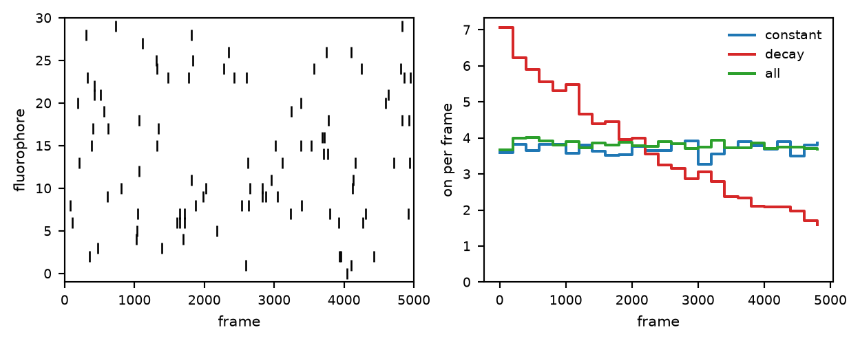
Left: the blinks of 30 fluorophores over the measurement (default settings, 5000 frames): each row one fluorophore, each tick a blink. Right: how many of 5000 fluorophores are on per frame, for the three choices of activation, with a bleaching probability of 0.3 and 2.5 blinks: decaying thins out as the fluorophores bleach, the other two stay flat.

4. Photons. Each blink gets a total number of photons, drawn at random around photons per blink with a spread of photons std. The fluorophore emits them at a steady rate while it is on, so each frame gets the share of the time it was on in it.

5. Drift, if add drift is ticked: the whole sample moves along a slow random path over the measurement, so every localization and every spot is off by where the sample was in its frame.

6a. Localizations. For each frame a fluorophore was on in, the number of photons detected is drawn around what it emitted (Poisson). Below the detection limit there is no localization. The rest are placed at the true position plus a random error whose size is the localization precision a good fit would reach – how precisely a spot of that many photons, on that background, can be located. The same precision is written into the table as xy_err_nm, so the reported error is honest: a plugin that checks precision against the data should find them equal. Two fluorophores on in the same frame closer than the separation would be one spot to a fitter; by default both are removed (close emitters).

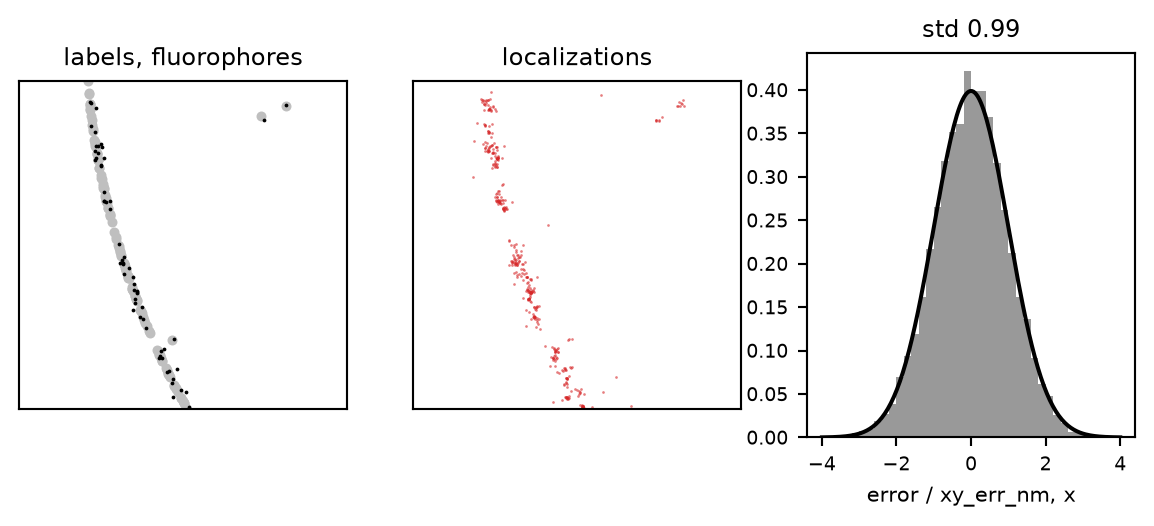
What a simulation of the demo gives, close up on the ring. Left: the labels (grey) and the fluorophores (black), at a labelling efficiency of 0.5 and a fixed linkage error of 10 nm: half the labels are empty, and a fluorophore sits near its label rather than on it. Middle: the localizations, a cloud around each fluorophore. Right: the error of each localization over the precision it reports, for those above 200 photons; it follows the standard normal (line), as an honest precision must.

6b. Camera frames. Here every spot is drawn onto a camera: the fluorophore's photons spread over the pixels as a Gaussian of the PSF sigma (astigmatic, whose shape changes with z, if astigmatic is ticked, or a measured PSF from a PSF calibration), on the background, with the camera's shot noise, read noise and gain. Nothing is removed, however dim or crowded: sorting that out is the fitter's job.

The frames are not written out as images. The plugin saves the simulation file, *.sim.yaml, which is the recipe – these settings and the seed – a few hundred bytes instead of hundreds of megabytes. Open it in a fitter as its file, as you would open a TIFF: the frames are drawn as the fitter reads them, identically every time, and the fitter takes the camera's pixel size, conversion and offset from it. Tick also write a TIFF for other software.

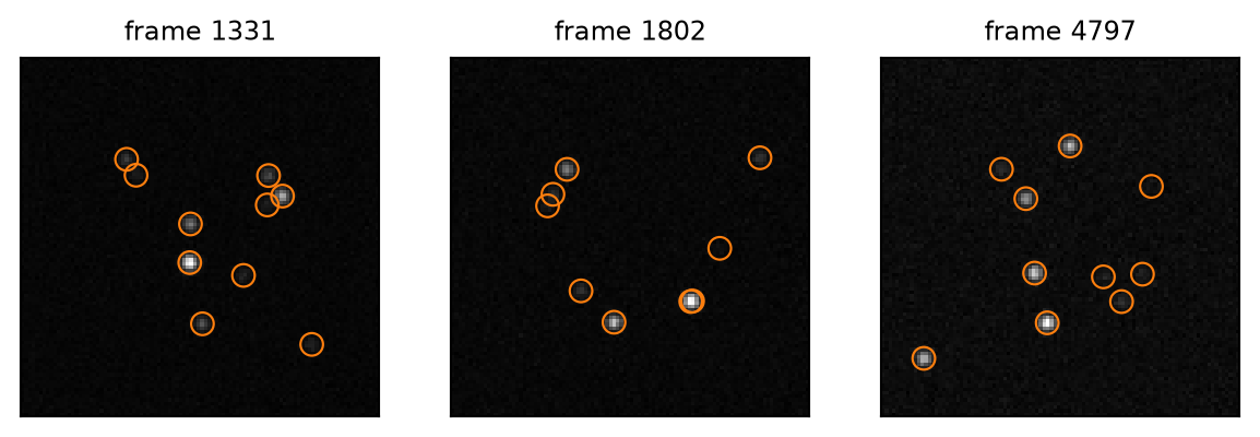
Three frames of the same simulation as camera frames (counts), with the true positions of the spots on in each marked. Some are dim – the start or end of a blink – and some overlap; all are drawn.

In detail

Sampling a structure. A line of length gets a Poisson number of labels with mean , uniform along it; a circle of radius gets on average; a polygon of area gets , uniform inside it, spread evenly over its z range; an image pixel of brightness (scaled so the brightest pixel is 1) gets for an image pixel of side . Every element can be blurred by its width, a Gaussian per axis. Explicit points are the same in every copy, the sampled elements are drawn afresh for each. Copies are placed uniformly in the field (with a min_distance between them, if given) or on a grid, turned in the plane (rotation: random) or in 3D (random_3d), tilted by up to tilt degrees, and moved by up to jitter nm. Each copy's position and turn are kept with the table, in metadata["copies"], by its number in the copy column, as angles with the rotation .

The off time from the number of blinks. A fluorophore blinks times before it bleaches, geometric with . Within a measurement of frames an unbleached one would be activated times, Poisson with mean . It shows blinks, whose mean is

falls as the off time grows, and the plugin finds the that makes equal to blinks by bisection. With the bleaching probability of 0.1 and 3 blinks wanted over 20 000 frames, the off time comes out at about 5600 frames. Setting off time directly overrides the calculation.

Spreading the blinks. With constant activation the blinks are first drawn at the fixed rate, then their start times are mapped, in order, onto as many times drawn uniformly over the measurement. The mapping keeps each fluorophore's own order, so its dark times come out longer early and shorter late – what raising the activation does. If a squeezed dark time would put a blink before the previous one had ended, it waits for the end. Every blink until bleached draws blinks with blinks and spreads them the same way, so the measurement's length plays no part.

Photons. The total of a blink is drawn from a gamma distribution with mean (photons per blink) and standard deviation (photons std): shape , which is never negative and is exactly when . The fluorophore emits it at the rate total / on time while it is on. So a blink much longer than average gives more than photons per blink, and a short one fewer.

The precision. The lateral precision per axis is that of a maximum-likelihood fit of a Gaussian spot (Mortensen et al. 2010, their eq. 5):

with the detected photons, the PSF sigma, the pixel size and the background in photons per pixel. Without background the integral is 0 and ; the more the background dominates, the closer the bracket comes to 0 and the larger the error. With EMCCD ticked the variance is doubled, the excess noise of the gain. The z precision is z precision times the lateral one (3 by default). With astigmatic ticked, is the spot's width at its z (the geometric mean of the x and y widths). The noise added to each position is drawn from exactly these precisions, and sigma_nm is the true width plus noise of the same size.

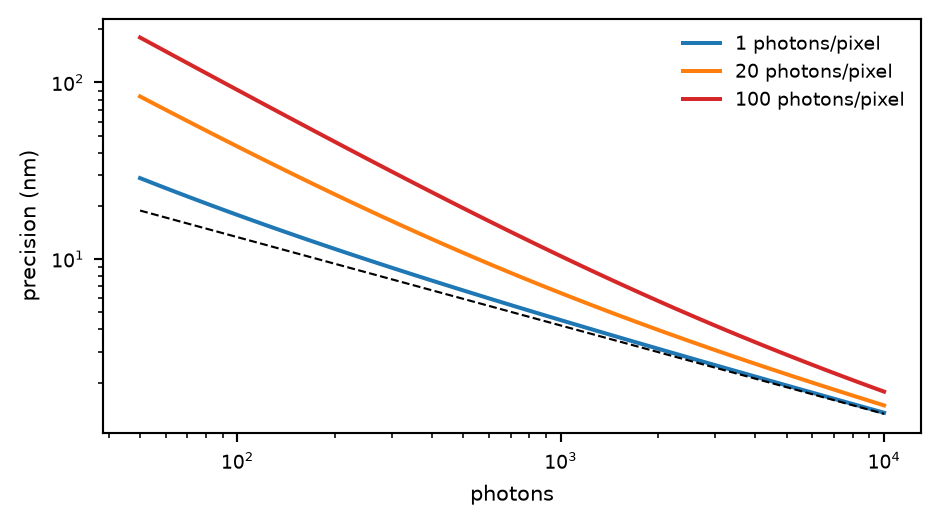
The Mortensen precision against photons for three backgrounds (PSF sigma 130 nm, pixels 100 nm), and the of no background at all (dashed). The background matters most for dim spots.

Close emitters. Localizations on in the same frame within the separation of each other are joined into groups, including chains of pairs. With remove both, every member of a group is dropped. With one localization, averaged, a group becomes one localization at the photon-weighted mean of its members, with their photons added, carrying the identity of the brightest and an n_merged column: what a single-emitter fit of an unresolved pair converges to.

The camera. A spot's photons are integrated over each pixel (the difference of error functions of the pixel's edges), and pixel is centred at pixel size, as the fitters assume. Behind a cylindrical lens each axis widens as a focused beam, and , the focal offset and the focal depth (Huang et al. 2008). The expected photons of each pixel, background included, are drawn as a Poisson count of electrons; with an EM gain that count is multiplied by a gamma of its size, which doubles the variance. The counts are electrons / conversion + offset plus Gaussian read noise, rounded and clipped to 16 bits. The background is flat over a frame, and with background std it varies from frame to frame. Each frame's noise has its own seed, so a frame is the same whichever block of the stack it is drawn in.

Drift. A random walk of 0.6 nm per frame and axis, plus a straight creep of 80, −50 and 30 nm in x, y and z over the whole measurement. It is added to the true positions, so localizations and frames drift alike, and the path is kept in metadata["drift_truth"], one row per frame, for comparing a drift correction with it.

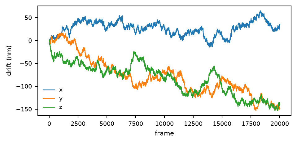
A drift path as add drift makes it, over 20 000 frames: the creep, with the random walk on top.

Parameters

Output

Localizations. A table in nanometres, replacing what is open:

• frame, x_nm, y_nm, z_nm, photons, background, xy_err_nm, z_err_nm and sigma_nm, as a fitter writes them;
• the truth: emitter (which fluorophore), dye (from the structure), copy (which copy of the structure), and n_merged when close emitters are averaged;
• in the metadata: the settings (simulation_settings), the numbers of labels, fluorophores and blinks, the off time that was used, each copy's position and turn (copies) and, with drift, the drift path (drift_truth).

The text says how many localizations came from how many fluorophores and blinks, the off time, and how many were too close together.

Camera frames. The simulation file; with also write a TIFF, the frames beside it; with load the truth, a table of every spot drawn: frame, the true x_nm, y_nm, z_nm (drift included), the photons it emitted in that frame, the background, emitter, dye, copy, and neighbour_nm, the distance to the nearest other spot on in the same frame.

Comparing with the truth. Ground Truth scores a table against its simulation. It needs no truth table: from a fit of a *.sim.yaml (the fitter writes the file into the table as its source) or from a simulated table (which carries its simulation_settings), it simulates the same molecules again and pairs each localization with its true spot. Because the precision is drawn honestly, a table simulated here should show an error over reported precision close to 1.

Differences from SMAP

Based on SMAP's ROIManager/Segment/SimulateSites (simulatelocs.m) and WorkflowModules/Loaders/SimulateCameraImages (simulatecamera.m) (Ries 2020). The physics within a blink is the same: an exponential on time starting anywhere in a frame, the photons shared by the time on, Poisson counts per frame, for an EMCCD and z three times the lateral precision.

• The precision. SMAP uses Mortensen's eq. 6, the error of an unweighted least-squares fit, with the PSF fixed at 100 nm. Here it is eq. 5, maximum likelihood, with the PSF sigma and pixel size set: it agrees with SMAPpy's own fitter to 1-2 %, where eq. 6 was 10-23 % too pessimistic.
• Blinking. SMAP's default model puts each fluorophore's blinks at independent random frames, their number drawn directly. Here the number follows from the off time and bleaching, set from the blinks wanted in the measurement. SMAP's "Dye" model is the option every blink until bleached; SMAP's version scrambles each fluorophore's order of blinks when it spreads them, this one keeps it.
• Photons per blink are gamma-distributed rather than normal and clipped at zero.
• Close emitters. SMAP keeps them in its localizations. Here they are removed or averaged, since a fitter could not have separated them; the camera frames keep them, as SMAP's do.
• Dim localizations. SMAP raises every count below 10 photons to 10 and keeps it; here a localization below the detection limit is not found.
• Structures are YAML files of elements and copies, placed at random or on a grid, rather than one site per ROI on a grid. An image is scaled by its brightest pixel, not by 255.
• Camera frames are a recipe drawn as they are read. SMAP Poisson-draws the photons for its localizations and then again for its frames, which doubles their variance; here they are drawn once.

References

• Mortensen KI, Churchman LS, Spudich JA, Flyvbjerg H. Optimized localization analysis for single-molecule tracking and super-resolution microscopy. Nat Methods 7, 377 (2010) – the precision, eq. 5. doi:10.1038/nmeth.1447
• Huang B, Wang W, Bates M, Zhuang X. Three-dimensional super-resolution imaging by stochastic optical reconstruction microscopy. Science 319, 810 (2008) – the astigmatic PSF. doi:10.1126/science.1153529
• Thevathasan JV, Kahnwald M, Cieśliński K, et al. Nuclear pores as versatile reference standards for quantitative superresolution microscopy. Nat Methods 16, 1045 (2019) – the geometry of the npc structure. doi:10.1038/s41592-019-0574-9
• Ries J. SMAP: a modular super-resolution microscopy analysis platform for SMLM data. Nat Methods 17, 870 (2020). doi:10.1038/s41592-020-0938-1