 .
.Analysis › Measure · version 3
The precision the data shows, beside the precision the fitter expected.
How well was a molecule placed? The fitter gives one answer for every localization: its precision, xy_err_nm, the Cramer-Rao bound (CRLB) computed from the photons, the background and the PSF. That number is what an ideal fit of an ideal spot could reach. It knows nothing of what happens after the fit: drift, vibration, a PSF that is not quite the model, a wrong camera calibration.
This plugin measures the precision on the data itself and puts it beside what the fitter claimed. It reports three kinds of number, and they are meant to disagree – the way they disagree is the diagnosis:
.By default it measures twice: the localizations as they are shown (the layer's filter and the ROI) and all of them, side by side (localizations). If nothing is filtered, it measures once.
What it needs. A frame column and positions for the pairwise displacement; a precision column (xy_err_nm, and z_err_nm for 3D) for the CRLB histogram and for comparing each pair with its bound; photons for the photon law (below). The displacement fit wants at least 200 pairs in the search radius. FRC wants at least 1000 localizations.
It always reads the ungrouped table, even when the layer shows the grouped one: grouping merges the repeated localizations of a blink into one, and those repeats are exactly what the pairwise displacement measures.
Photons and on-times are described by Localization Statistics, which fits the same model to the precision histogram as this plugin does.
1. Pairs. For every localization, every localization in the next frame within the search radius is paired with it – not only the nearest one. By default the radius is 6 times the median precision. In 3D the search is a cylinder: the disc laterally, and within the axial search in z (6 times the median axial precision by default).
2. Signal and background. Most pairs are one molecule seen twice. Some are two different molecules that happen to be close. Those are spread evenly over the search disc, so their share of the distance histogram rises in a straight line with the distance  . The pairs of one molecule follow a known curve instead: if each localization is off by a random error of size
  in x and in y, the distance between two of them has the density
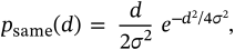
which peaks at  . The plugin fits the sum of the two curves, the fraction
  of same-molecule pairs and
  together. The fit is maximum likelihood on the distances themselves, so the histogram's bins change nothing but the picture.
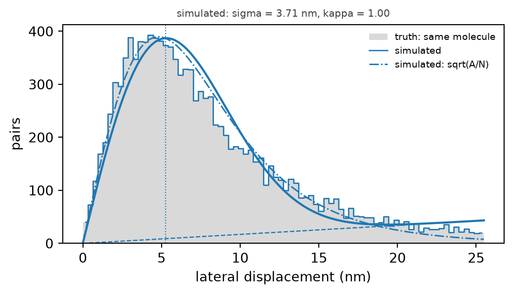
The distances between localizations in consecutive frames of a simulated dataset (blue steps), and the fit: the whole model (solid), its background of different molecules (dashed), the peak at  (dotted), and the photon law (dash-dot, step 3). Grey: the pairs the simulation knows are one molecule – nearly all of them. The single
  misses the long tail of dim pairs and hands it to the background; the photon law, with a width per pair, follows it.
3. The pairs are not a typical localization, so the photons are used too. A single  describes the pairs only if every localization is equally good. In real data some are bright and some are dim, and the pairs are a particular subset of them: the frames of a blink that is on in two frames in a row. So the plugin fits the same distances twice more, each time letting every pair have its own expected width:
 with the photon count
  , and one number
  is fitted for all pairs. The law can then say what a localization of any brightness is worth – in particular the median one of the table, which the text reports. It needs no camera calibration: a wrong gain changes
  and
and  by opposite factors and leaves
  where it was.
 , says how far the data misses the fitter's own bound.
  : the fitter reaches its bound and the photon calibration is consistent with the data.
  : something is worse than the model says – a wrong gain or offset, a PSF that does not match, residual motion.
  does not say which.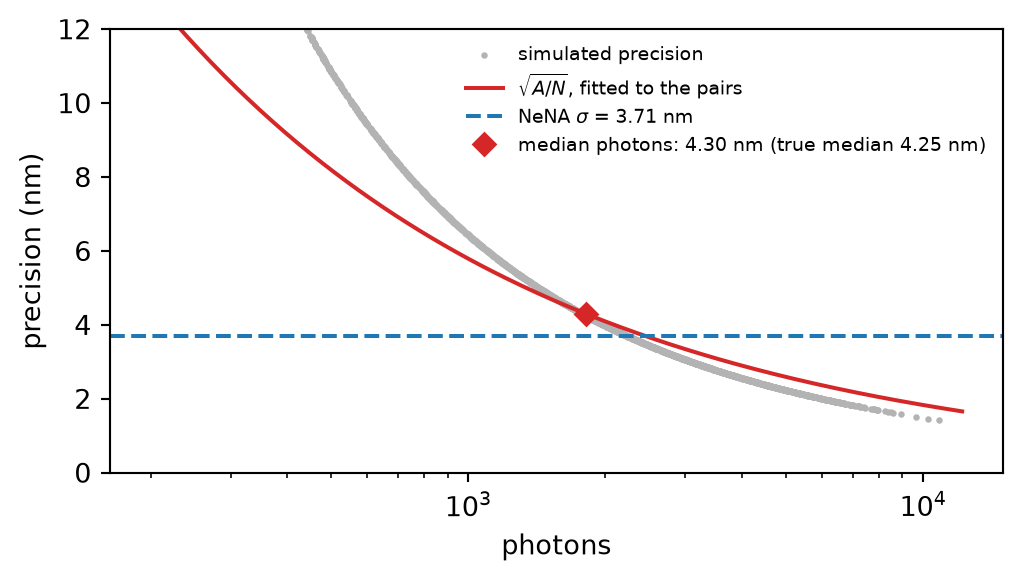
What the photon law says each localization is worth (red), against the true precision of each localization of the simulation (grey dots). The plain NeNA  (blue) is one number for all of them. Diamond: the law at the median photon count, which is what the text reports.
4. Per axis. The same mixture is fitted to the signed displacements in x, in y and, for 3D data, in z, each on its own. This is how the axial precision is measured: the z fit needs no model of how the PSF changes with depth. The mean of each displacement is printed as well: it is the drift over one frame.
5. Frame gap. The whole fit is repeated for localizations 2, 3, ... up to frame gaps to frames apart. If nothing moves, a molecule is placed just as well two frames later and  stays flat. If the sample drifts or vibrates, the displacement grows with the time between the two localizations, and so does
  . A straight line through
  against the gap, extrapolated to gap zero, gives the precision with the motion taken out, and its slope gives how far the sample moves per frame. After drift correction, a rising curve says the correction missed the fast part of the motion – which nothing else in the program shows.
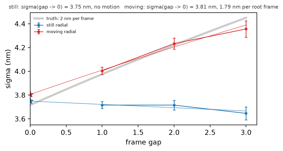
 against the frame gap for the simulated data as it is (blue) and with a random walk of 2 nm per frame per axis added to every position (red). The star is the extrapolation to gap zero. Grey: what the walk that was put in should give.
6. The CRLB histogram. The precision column is histogrammed and the distribution that exponentially distributed photons imply is fitted over it, exactly as in Localization Statistics: the single number  is the precision at the mean photon count. The pairwise
  is drawn over it as a dashed line, which is the comparison the plugin exists for.
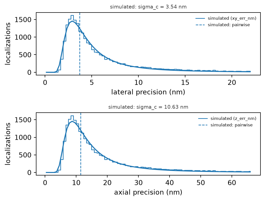
The CRLB histograms of the simulation, lateral and axial, with the fitted distribution (solid) and the  the pairs measured (dashed).
7. FRC. The frames are cut into FRC blocks – equal stretches of the acquisition – and the blocks are dealt at random into two halves, so that all the frames of one blink land in the same half. Both halves are rendered, and their Fourier transforms are compared ring by ring: the correlation is 1 at coarse detail, where the two images agree, and falls to 0 at fine detail, where each shows only its own noise. The resolution is where the smoothed curve first falls below 1/7, the threshold of Nieuwenhuizen et al. This is done FRC splits times with different deals; the curves are averaged, and the spread of the resolutions is the error bar.
Drawn beside it, dashed, is what the blur of the measured precision alone leaves of the correlation. It is not a fit.
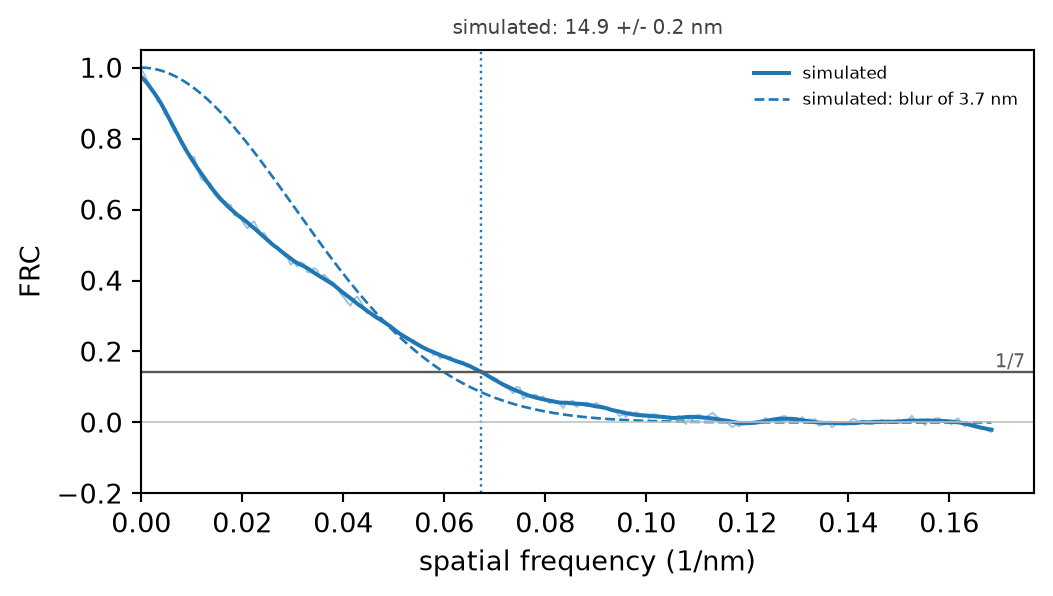
The FRC of the simulation (the light line raw, the dark one smoothed), the 1/7 threshold, and the blur that the pairwise precision alone implies (dashed).
The pair model. Two localizations of one molecule are at the same true place, so their displacement is the difference of two independent errors: a variance  per axis. The lateral distance
  of a pair follows Churchman's law at zero true distance, truncated at the search radius
  , mixed with the uniform background:

Per axis it is a truncated Gaussian of variance  on a background that is the chord of the search disc,
  , for x and y, and flat for z (the search is a slab of
  the axial search there). Displacements are later minus earlier, so their mean is the drift over the gap; the fit ignores the mean.
Why all pairs, not the nearest neighbour. With every pair inside the radius, the pairs of different molecules are uniform in the disc and their density is exactly  . Keeping only the nearest neighbour makes that background depend on the density of the sample: a molecule with a close neighbour hides its true partner.
The scaled fits. For the photon law each pair has its own variance  , for the CRLB fit
  , with
  the photons and
  the precision column of the two members. The density is the same mixture, one Rayleigh per pair. The photon law assumes shot noise dominates; with a heavy background the dim end wants an extra term in
  , and that is where a deviation from the law shows (the red curve above, at the dim end).
The fit. Maximum likelihood, by a Nelder-Mead simplex in  , so neither can leave its range. It starts from three signal fractions (0.5, 0.15 and 0.85) and keeps the best, then restarts the simplex once at its own optimum, because on a shallow valley a simplex stops early and would remember where it started. The error is from the curvature of the log-likelihood in both parameters together; if that comes out singular it falls back to
  for
for  pairs. Fewer than 200 pairs are not fitted, and a fit in which fewer than 100 pairs are signal says so.
The frame gap line. A random walk of step  per frame and axis adds
  to the displacement variance over
  frames, so
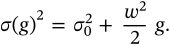
The line is fitted to  by weighted least squares, each gap weighted by its fitted error;
  is its intercept and
  is printed as the motion "per root frame". The slope counts as motion only when it is more than twice its own standard error (from the same weighted fit) above zero; otherwise the text says there is no motion beyond the scatter of the gaps and
  is 0. Five points that scatter by their errors always have some slope, and on still simulated data it came out as half a nanometre per root frame before this test.
The CRLB histogram fit is Localization Statistics' least-squares fit of  ,
,  , to the histogram from zero to its 99.5th percentile. If
  lands outside 0.3 to 3 times the median, the photons are not exponential and the text says to read the median instead. When the selection is measured and the layer's filter cuts the precision column, the histogram is fitted between the cuts only: a lower cut would otherwise leave empty bins the model reads as a distribution moved up (11.3 nm for a true 8.9 nm, with a cut at 7 nm), and the fit of the part that survived recovers the whole.
FRC. With the half-images  and
and  , the correlation over a ring of spatial frequency
  is
is
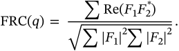
The images are tapered at the edges first (a Tukey window over the outer eighth), and the curve is smoothed with a Savitzky-Golay filter before the crossing is read. The picture is transformed in tiles of 512 pixels whose sums are added, so the pixel can be small whatever the size of the field; tiles with fewer than 200 localizations are skipped. With the FRC pixel at 0 the resolution is first measured on a coarse grid (the field over 1024 pixels) and then again with a pixel a fifth of what that found. A coarse pixel cannot see a resolution finer than about two of it, so when the coarse curve never falls through 1/7 the coarse pass is repeated at a quarter of the pixel, down to 1 nm. The blur envelope is  , and the text reports where it alone crosses 1/7, at
  . That is not a limit on the FRC: a structure localized many times per molecule resolves better than it, a sparsely labelled one worse.
FRC per axis (3D). Instead of rings of a 2D picture, planes of the 3D transform perpendicular to one axis (a Fourier plane correlation) give a resolution along x, y and z separately, each plane summed only over the band of frequencies the other two axes resolve. The volume is far sparser than the projection, so the lateral numbers come out worse than the ring FRC, often by a factor of two; they are the ones to quote for a 3D measurement.
A ROI or a slab costs only the pairs that straddle its edge, which for a search radius of tens of nanometres is nothing – except in z, where a slab (a filter on z_nm, or the 3D view's slab while plugins use it) thinner than four axial precisions loses the partners that fell outside and  reads low; the text warns. The pairs within one frame gap are searched with one KD-tree per frame.
Compared with the papers. NeNA (Endesfelder et al. 2014) estimates the precision from nearest neighbours. Here:
 (above);
 (NeNA) fit, because the pairs are the frames in which a blink began or ended and are not a typical localization (step 3).
FRC follows Nieuwenhuizen et al. 2013, with the fixed threshold of 1/7, and departs in three places:
| setting | default | what it does |
|---|---|---|
localizationssource | both, side by side | What the image is worth, what the sample is worth, or the two compared. as plotted answers "how well is what I am looking at placed", all "how good is this sample". A filter on precision or photons does not bias the pairwise fit, it selects: both partners of a pair must survive it, and the first and last frames of a blink are the dim ones, so a hard cut removes true pairs preferentially. The fitted signal fraction shows it; |
pairwise displacement (NeNA)pairwise | on | The experimental precision, from molecules localized in more than one frame. It is the only one of the three methods that sees drift, vibration and a wrong calibration, and the only one that needs molecules on in consecutive frames. |
CRLB histogramcrlb | on | What the fitter expected, from the photons. Needs a precision column; without one the histogram is left out. |
FRC resolutionfrc | on | What the picture resolves: the localization error, the labeling density and the drift together. The slowest part of a run on a large field; untick it when only the precision is wanted. |
frame gaps tomax_gap | 5 | The fit is repeated at every gap up to this: flat means nothing moved between frames. 5 is enough to see a trend. At long gaps fewer molecules are still on, so the pairs thin out and the error bars grow. 1 to 50 |
search radiusreach_nm | 0 nm | 0: 6 x the median precision. The peak sits at |
axial search (more)reach_z_nm | 0 nm | 3D data only. 0: 6 x the median axial precision. Kept narrower than four axial precisions, it cuts off the tail of the z displacements and |
FRC per axis (3D)frc_axes | off | The resolution along x, y and z separately, from planes of the 3D transform rather than rings of a 2D one. 3D data, and a ROI rather than a whole field of view. The volume is transformed tile by tile, each tile the full depth of the data, so a whole field of view is many tiles and a long run. |
FRC blocks (more)frc_blocks | 20 | The acquisition is cut into this many stretches of frames before the two halves are dealt, so that a blink stays whole. More blocks mix the two halves more evenly over the acquisition, which matters when the sample changes over time; fewer keep more blinks whole. at least 2 |
FRC splits (more)frc_repeats | 5 | The curves of this many random deals are averaged, and their spread is the error bar. At least 3 are needed for the spread to be the error bar; with fewer, the error comes from the ring statistics of the curve alone. 1 to 50 |
FRC pixel (more)frc_pixel_nm | 0 nm | 0: measured roughly first, then at a fifth of that resolution. Leave it at 0 unless two measurements must be compared at the same pixel. A pixel coarser than about a fifth of the resolution reads the resolution too large; one much finer only costs time. |
bins (more)bins | 80 | Drawing only: every fit is on the displacements. at least 10 |
frames per gap (more)max_frame_pairs | 20000 | A longer movie is sampled evenly across its whole length. Only a speed limit: the default covers most acquisitions whole. at least 100 |
pairs per gap (more)max_pairs | 2000000 | More pairs than this at one gap are thinned to a random sample of this many. at least 1000 |
seed (more)seed | 0 | Which pairs are kept when there are more than the limit. |
The text has one block per set of localizations, a line per number:
 and the median of the precision column, lateral and axial.
 at gap 1, the number of pairs and the percentage in its peak (the signal fraction
  , see below); then
  ,
,  ,
,  and the mean shift over one frame.
 and the percentage of pairs that are one molecule by this fit, and what it gives for the median paired localization and for the median localization of the table.
 alone crosses 1/7; per axis: the resolutions and the axial-to-lateral ratio.
 and the motion per root frame, or that there is no motion beyond the scatter of the gaps.
A table in pixels (x_pix, xy_err_pix) is measured and reported in pixels.
Besides the text:
 against the frame gap (when frame gaps to is above 1), FRC, FRC per axis, and the CRLB histograms.
Reading them. Pairwise  close to the CRLB median and
  near 1: the data are as good as the fitter says.
  well above 1: the fitter's precision is optimistic – check the camera gain and offset, the PSF model, and the frame-gap curve for motion. A flat gap curve means nothing moved; a rising one, residual drift or vibration. An FRC curve that falls well before the dashed blur envelope means the picture is limited by labelling density, drift or too few localizations, and better precision would not help; if the two fall together, the precision is what limits it.
The percentage in the pairwise line is a property of the single- model, not a count. When the precisions vary, as they always do, the one Rayleigh describes the core of the distribution and hands part of the broad tail of dim pairs to the background: in the simulation above all but a few tenths of a percent of the pairs are one molecule, and about 85% are in the single
  's peak. The photon law, which gives every pair its own width, finds a fraction close to one, and that is the one the law line reports.
The FRC is based on SMAP's Analyze/measure/FRCresolution, and the CRLB histogram on its Analyze/measure/Locstatistics (Ries 2020); the pairwise displacement (NeNA) and the comparison with the CRLB are new.
 .
. scaling.
 survives a cut better than the plain
  .
. times the precision, and the background must be visible beyond the tail for the fit to tell them apart. Much wider costs time and adds background; narrower than about three times the precision cuts into the signal. In a very dense sample a smaller radius keeps the background share down.
 reads low; the text warns.