File › Load · version 2
Read a MINFLUX .npy, .zip or .json export.
Opens the localizations exported by an Abberior MINFLUX microscope (Gwosch et al. 2020), so that they can be filtered, rendered and analysed like any other table.
MINFLUX (Balzarotti et al. 2017) does not take camera frames. It finds a molecule by probing it with a beam that has a dark centre, in several iterations, each one closer and more precise than the last, and records every iteration of every localization. The export is a list of those records. This plugin takes the last iteration of each valid one.
It reads the three shapes the export comes in: a .npy file (a NumPy structured array), a .json file with the same nesting, and a .zip that holds either. It does not read MINFLUX data saved as a MATLAB .mat file.
1. The last iteration. Of the iterations of a localization only the last, the most precise, is kept. Its position is converted from metres to nanometres (x_nm, y_nm, and z_nm if any localization has a z).
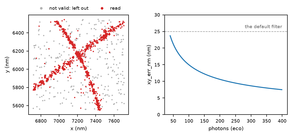
2. Valid ones only. The instrument marks each localization valid or not (vld), by criteria set in its own software. Those that are not, and any with no position in the last iteration, are left out.
3. Sorted by time. MINFLUX has no frames. The localizations are put in the order they were taken (tim), and frame is the rank in that order: 0 for the first, 1 for the next, and so on. The clock itself is kept in time_s, in seconds, and the trace a localization belongs to in tid.
4. Photons and precision. The photon count is the last iteration's eco. The precision is not in the export, so it is estimated from the photons (see In detail), as SMAP does.
Left: a simulated MINFLUX export, read. The localizations the instrument marked valid are read (red); those it did not are left out (grey). Right: the precision given to each localization, from its photon count alone.
The precision. With  the photons of the last iteration, the lateral precision is set to
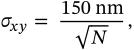
SMAP's number for the json export. It is a stand-in so that rendering and the precision filter have something to work with, not the precision of a MINFLUX localization, which depends on the beam pattern and is usually several times better. sigma_nm is set to 150 nm for every localization, for the same reason. With the default filter of 25 nm on xy_err_nm, localizations with fewer than 36 photons are hidden when the file opens.
The columns.
| column | from the export |
|---|---|
x_nm, y_nm, z_nm | loc of the last iteration, times  |
frame | the rank in time |
time_s | tim |
tid | tid, the trace |
photons | eco |
efo, cfr, dcr, efc, ecc, fbg | the same, where the export has them |
iteration | itr, the number of the last iteration |
Grouping by trace. The instrument has already said which localizations belong to one molecule: those of one trace, tid. So the grouped table has one row per trace – its mean position, its summed photons, its first frame, and in n_in_group how many localizations it had – rather than the distance-and-frame linking of a camera file, which would cut a trace wherever it wandered 50 nm between two localizations. Before version 2 it was linked like a camera file. To look at every localization, untick grouped on the layer.
Positions are kept as the instrument gives them; they are not shifted to start at zero. The file's entry in the session (metadata["files"]) records a nominal pixel size of 100 nm, as SMAP does; there is no camera.
The table, added to the session as a file of its own. The text says how many localizations were read.
Based on SMAP's Loader_minflux_json (Ries 2020). The main changes:
.npy and .zip exports are read, the MATLAB .mat export is not. for every export. SMAP uses it for the json export, and for a
 .mat export works it out from the size of the last iteration's beam pattern instead.| setting | default | what it does |
|---|---|---|
filepath | – | The localization file to read. |
add to the open filesappend | off | Join the table as one more file instead of replacing everything; this is File > Add file. |