Line Profile

Analysis › Measure · version 4 · has a preview · can run live

Profiles along or across a line ROI, fitted without binning them.

What it does

Many questions about a super-resolved image come down to a line drawn over it: how far apart are the two membranes of the nuclear envelope, how wide is this filament, where does this labelled region end, how large is this vesicle. Line Profile answers them. It takes the localizations inside a line ROI, lays them out along the line (or across it, or in z), and fits a model of the structure to them: one peak, two peaks a distance apart, an edge, a filled disk or a ring. The numbers that come back – a distance, a width, a radius – come with error bars and with a score that says which model the data prefers.

It differs from reading a histogram by eye, or fitting one, in three ways that matter when there are few localizations:

It fits the localizations themselves, not a histogram of them. No number it reports depends on a bin width.
It knows how precisely each localization was measured, and takes that blur out, so a width is the width of the structure rather than of its blurred picture.
A flat background of unspecific localizations is part of every model, so a few stray points do not widen a peak.

A line is usually drawn over two channels, and what is wanted is how they differ, so each visible layer is fitted on its own and drawn in its own colour.

What it needs. A line ROI, drawn in the render window, with a width wide enough to take in the structure. At least 8 localizations per layer (a layer with fewer is skipped, and a single layer with fewer is refused); below 30 the fit still stands, but its error bars are too optimistic and the bootstrap (below) is the one to read. The localization precision xy_err_nm (for a z profile, z_err_nm) is used when the table has it; without it one width is fitted for all localizations, and the text says so.

The fit takes tens of milliseconds, so the plugin offers a live tick: the profile is refitted while the line is dragged, which makes it a tool one can aim with.

How it works

1. The line's own coordinates. Every localization inside the ROI is given two new coordinates: how far along the line it lies, measured from the end where the line was started, and how far across it, measured from the line's centre, positive to its left. Localizations outside the ROI's rectangle are left out.

2. One profile. One of those coordinates is fitted (profile). Along the line is the default and the usual case: the line is drawn across the structure, and the profile along it is the structure laid out under the line – two membranes become two peaks. Across the line is the profile of something the line runs along, such as the width of a filament the line was drawn on. z is the depth of the same localizations.

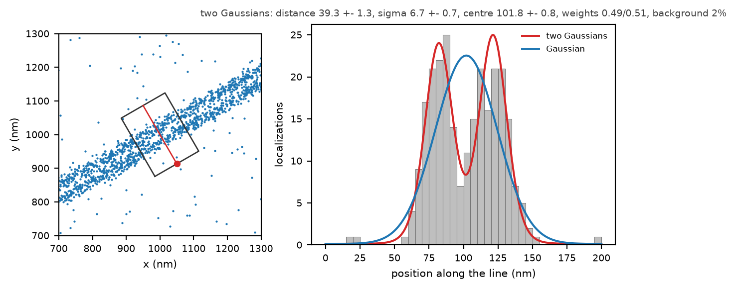
Left: two filaments 40 nm apart with a few stray localizations, and a line ROI drawn across them (the start of the line is the dot). Right: the profile along the line, with the two models the plugin fitted to it. The histogram is only for the eye; the fits are to the localizations.

3. A model of the structure. The plugin fits one of five shapes (model), or all five for a comparison:

Gaussian – one thin structure: a filament, a membrane seen edge-on. It gives a centre and a width.
two Gaussians – two structures of the same width a distance apart, such as the two membranes of the nuclear envelope. It gives the distance, the shared width, the centre between the two and how the localizations are shared between them.
step – an edge: uniformly labelled on one side, empty on the other. It gives where the edge is and how sharp. Which side is full is not guessed: both are fitted and the better one kept.
disk – a uniformly filled circle, seen from the side.
ring – the outline of a circle, seen from the side: the profile with a horn at each end that a vesicle or a nuclear pore gives.

Disk and ring give a centre and a radius. Every model also has a flat background, a fraction of localizations spread evenly over the ROI (uniform background).

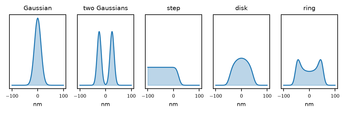
The five shapes on a 200 nm window, each blurred by 8 nm, with no background. The step is the only one that does not come back to zero: it is a region filled up to an edge.

4. Each localization carries its own blur. A localization is not a point: its position is known to within its precision, typically 5 to 15 nm. What a histogram shows is the structure blurred by those errors, so a 6 nm wide membrane measured with 8 nm precision looks 10 nm wide. With use localization precision on, the model is blurred for each localization by that localization's own precision, and the width that is fitted is the width of the structure itself.

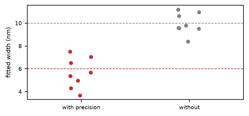
The width of each of the two structures, fitted to eight simulated profiles (200 localizations, 40 nm apart, structures 6 nm wide, precisions around 8 nm). With the precisions (red) the fitted widths scatter around the structure's own width; without them (grey) it measures the width of its blurred picture, 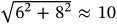nm.

5. Fitting without bins. The model is a probability: how likely a localization is to sit at each position along the ROI. The fit looks for the parameters under which the localizations that were actually found are most probable – the maximum likelihood estimate. No histogram is involved, so no fitted number depends on a bin width; the bars in the figure are only for the eye. Because the probability is spread over the ROI's own extent, a structure cut off by the end of the ROI is not biased by the cut. The old way, a least-squares fit to a histogram, is available as binned for comparison.

6. Starting where the data is. A fit finds the best answer near where it starts. Started badly, a two-Gaussian fit can settle on both peaks sitting on top of each other and report a distance of zero, which looks like an answer. So the starting values are read off the data: the peak and its half-maximum width from a coarse, smoothed histogram, and for the two Gaussians a preliminary fit by expectation-maximization that pulls two components apart wherever two describe the data better. That preliminary fit is started three ways – on the two ends of the tallest peak, on the two highest separate peaks, and as far apart as the data goes – each once with the width read off the profile and once much narrower, and the best one is kept. The narrow start matters for a close pair: its profile looks like one broad peak, and a start as wide as that peak can only shrink onto it.

7. One structure or two? Two Gaussians always fit at least as well as one, because they can become one. The question is whether they fit enough better to justify the extra parameters. That is what the AIC (Akaike information criterion) measures: the fit's likelihood with a penalty for every parameter. Lower is better. With model set to all five, compared, every model is fitted and they are listed best first by AIC.

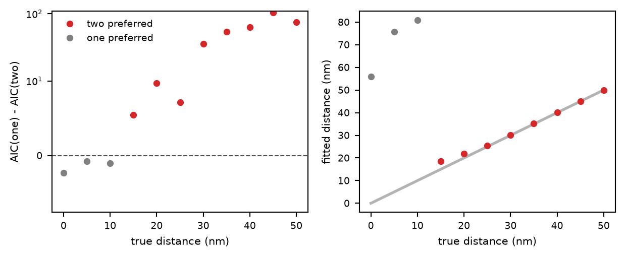
Eleven simulated pairs of structures, 0 to 50 nm apart (200 localizations each, structures 6 nm wide, precisions around 8 nm). Left: how much lower the AIC of two Gaussians is than that of one; above the dashed line two are preferred. Right: the distance the two-Gaussian fit returned, against the truth (line). Where two are preferred (red), the distance comes back. Where one is (grey), the two-Gaussian distance means nothing – below about 15 nm the pair is not resolved, and the second component wanders off onto the background. Near the resolution limit a pair can also be missed, both components settling on one broad peak: a distance of zero there is worth a second look.

8. How sure is the answer. Every number comes with an error bar, worked out from how sharply the likelihood falls off around its best value. That is the standard approximation, and it is good when there are many localizations. With few – below about fifty – it is too optimistic. The bootstrap (bootstrap, the number of resamples) is the honest alternative: it draws, many times over, a new set of the same number of localizations from the ones there are (some twice, some not at all), fits each, and reports the range that holds most of the answers (confidence, 95%). It assumes nothing about the shape of the uncertainty, and it shows when a width runs into zero or a distance is not really resolved.

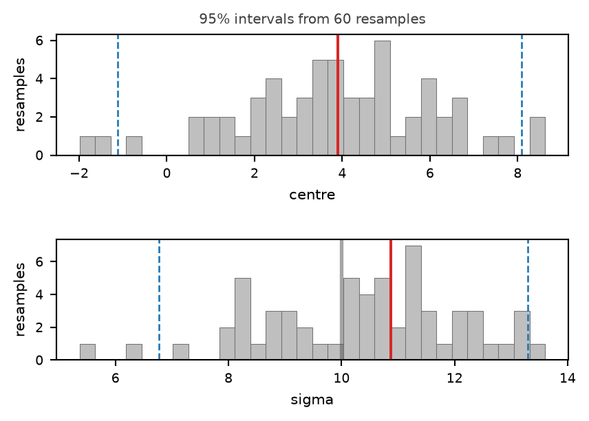
The bootstrap of a Gaussian fitted to only 40 localizations of a structure 10 nm wide (60 resamples). Red: the fit; dashed blue: the 95% interval; grey: the true width. The width's interval reaches further below the fit than above it, which a single error bar cannot say.

In detail

Coordinates. With the line's ends and (the midpoints of the ROI rectangle's short sides), its length and unit direction , a localization at has

along and across. The windows are and , the ROI's width; with a length the along window becomes , centred on the line, and localizations outside it are dropped from every profile. The z window is the first layer's filter on z_nm, in nanometres; a side the filter leaves open – or both, without a filter or a session – is the data's outermost value widened by 5% of the range. It matters, because it is part of the likelihood.

The likelihood. For the fitted coordinates in a window of length , and a model density normalised over that window, the fit maximises

with the background fraction, . The subscript on is the per-localization blur: every width of the structure enters localization 's density as

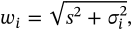
its precision (xy_err_nm or xy_err_pix, z_err_nm for z). A missing or non-positive precision is replaced by the median of the others; without precisions, for all. The maximum is found with L-BFGS-B within bounds: a centre or an edge inside the window, a width, distance or radius between 0 and , a fraction between 0 and 1.

Widths as variances. Near , is flat in , so is a stationary point whatever the data, and a gradient method started above it can walk down to it and stop, reporting a structure of no width. Every width is therefore fitted as its square , in which that point has a slope.

The densities. With and the standard normal density and cumulative distribution, the Gaussian is truncated to the window,

and the other shapes are built from it or from :

Two Gaussians: times a Gaussian at plus times one at , one shared width .
Step: , normalised by its integral over the window in closed form, from with . Rising and falling are both fitted; the likelier is kept.
Ring and disk: seen edge-on, a circle of radius puts its mass at . For a ring the mass is uniform in ; for a filled disk it goes as . In the angle neither has the singularity that the projected profile has at , so each is a weighted sum of truncated Gaussians at , at the nodes of Gauss-Legendre quadrature over . The number of nodes is , the median blur, kept between 32 and 128, so that a sharp shape is not drawn as ripples.

Starting values. All read off a histogram of bins over the window, smoothed with the kernel :

the peak is the centroid of the contiguous run of bins above half the maximum, weighted by how far above half each is;
the observed width is that run's full width at half maximum over 2.355, and the structure's width to start from is , the median precision, but not less than ;
the edge of a step is where the profile, walked in from the fullest bin of the plateau, first falls below half the plateau; the plateau is the 75th percentile of the third of the bins on the full side;
disk and ring start with a radius of half the half-maximum span;
the background starts at 5%, or, for two Gaussians, at the share EM gave it.

Expectation-maximization for two Gaussians alternates between assigning each localization to the two peaks and a flat background component (density ) in proportion to how well each explains it – the responsibilities – and refitting each component to what it was given. The means are weighted by precision, and the shared structural variance has the precisions taken out:

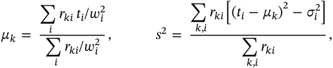
with floored at 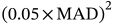, MAD the robust spread . At most 200 rounds, until the parameters move by less than . The three starts are the half-maximum ends of the tallest peak; the two highest maxima of the smoothed profile that have a dip below four fifths of the lower one between them; and the 15th and 85th percentiles. Each is run at the width read off the profile and at a third of it, and the run with the highest mixture likelihood is kept. EM ignores the truncation at the window, which is why it is a start and not the answer.

Model comparison. With free parameters (the model's, plus one for the background when it is fitted) and localizations,

Both are reported; the models are ranked by AIC. BIC penalises every parameter more than AIC does whenever , which is always here.

Error bars. The Hessian of at the maximum – the observed Fisher information – is taken by central differences, with a step of in each parameter. A parameter that ended on its bound (a width at zero, a background at nothing) has no error bar and is left out; the rest are of the remaining block, and a width's error is carried back from its variance, .

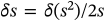The bootstrap. Each resample draws localizations with replacement, each keeping its own precision, and refits the same model starting from the full fit's parameters, with the step facing the same way. The interval is the percentile interval: for 95%, the 2.5th and 97.5th percentiles of the resampled values. Resamples that fail to fit are dropped; if fewer than half succeed, no interval is given. The percentile interval is the simplest one and slightly undercovers a width on a small sample: on twenty-five simulated profiles of forty localizations, a nominal 95% interval on the width held the true value 22 times. Only the best model is resampled.

Binned. With fit set to binned, the parameters minimise over the histogram bins of width bin, the counts the model predicts in the bin – its density integrated over the bin, by three-point Gauss-Legendre quadrature (for per-localization precisions, the density averaged over the sample's precisions). The log-likelihood that is reported is still the unbinned one at those parameters, so the two methods and all models are compared on the same scale.

Parameters

setting	default	what it does
profile `axis`	along the line	Which coordinate is histogrammed and fitted. Along is what a line is usually drawn for – the structure laid out under it; across measures the width of something the line crosses. For a z profile, the table needs `z_nm`; its precision is `z_err_nm`. Choices: along the line; across the line; z
localizations `source`	each visible layer, in its colour	A line is nearly always drawn over two channels and the measurement is how they differ, so a profile per layer is the usual thing; SMAP's lineprofile does the same. Choices: each visible layer, in its colour; the selection, as one
model `model`	Gaussian	What the profile is expected to be. All five, compared is the way to find out which shape the data supports; then fit that one alone. Choices: Gaussian; two Gaussians (a distance); step (error function); disk, seen edge-on; ring, seen edge-on; all five, compared
fit `method`	unbinned, maximum likelihood	The unbinned fit uses the localizations themselves, so no fitted number depends on the bin width; with few localizations it is the only one worth trusting. Binned is there to compare with SMAP and older results. Its answer moves with bin. Choices: unbinned, maximum likelihood; binned, least squares
use localization precision `use_precision`	on	Each localization is a Gaussian of its own precision, so the fitted width is the structure's rather than the picture's. Leave it on. Off, the fitted widths include the localization error, which is what SMAP's line profile reported.
uniform background `background`	on	A flat fraction of unspecific localizations; without it a Gaussian asked to explain them comes back too wide. Off only when the ROI is known to hold nothing but the structure: one parameter fewer to estimate, which helps a very small sample.
bootstrap `bootstrap`	0	0: off. Otherwise this many resamples of the localizations, for confidence intervals that assume nothing about the shape of the likelihood – what to use below ~50 localizations, where the fit's own error bars are optimistic. A few hundred resamples. Each is a full fit, so 200 resamples of the two Gaussians take around ten seconds, and live becomes slow with it on. 0 to 5000
confidence (more) `confidence`	95 %	The interval the resamples are asked for. 50 to 99.9 %
bin `bin_nm`	0 nm	0: chosen from the data. In pixels for a table in pixels. Drawing only, unless the binned fit is chosen. The automatic bin follows the Freedman-Diaconis rule, , kept between 1/200 and 1/5 of the window.
length (more) `length_nm`	0 nm	0: the ROI's own length. Otherwise a window of this length centred on it, so two ROIs can be compared directly. Also useful to keep a long line's profile to the part around the structure.

Output

The text gives, per layer and per model, the fitted values with their error bars (a value printed without one usually ended on its bound), the background fraction, the log-likelihood, AIC and BIC. With several models, the best by AIC is named and by how much. With the bootstrap on, the interval of every parameter of the best model.
The profile: the histogram with the fitted curves. With one layer, every model fitted is drawn and the best is red; with several layers, each is drawn in its layer's colour with only its best model. The curve is the density scaled to the histogram, and it is a fit to the localizations, not to the bars – it can sit over an empty bin with nothing wrong.
The scatter: the localizations in the line's coordinates, across (and z, when there is one) against along. A projection hides things – a filament that leaves the ROI half way, two structures that cross – and the scatter shows them.
The bootstrap, when it was run: the resampled values of each parameter of each layer's best model, with the fit and the interval – one tab per layer.

A good result has a curve that follows the histogram, an error bar well below the value, and, for a distance, an AIC clearly in favour of two Gaussians. A distance whose bootstrap piles up at zero, or a width with no error bar, has not been measured: the data do not resolve it.

Differences from SMAP

Based on SMAP's Analyze/measure/lineprofile (Ries 2020), which makes a histogram of the ROI with a fixed bin width (2 nm, or the render pixel size) and fits it by least squares. Here:

Unbinned maximum likelihood replaces the least-squares fit to a histogram: with few localizations the bin width moves the answer by more than its error bar.
Each localization's own precision is folded into the model. SMAP either fits one width for everything or fixes it to the median precision (sigma=<locp>).
A flat background is a fraction of the localizations, fitted with every model. SMAP's models are curves with an amplitude and a constant offset, fitted to the counts; here every model is a probability density over the ROI, which is what makes the models comparable by their likelihood.
The step is a single edge. SMAP's Flat is a top hat of fitted length – two edges; here an edge is fitted on its own, which does not need the other end of the structure to be in the ROI.

References

Akaike H. A new look at the statistical model identification. IEEE Trans Automat Contr 19, 716 (1974). doi:10.1109/TAC.1974.1100705 – the AIC.
Dempster AP, Laird NM, Rubin DB. Maximum likelihood from incomplete data via the EM algorithm. J R Stat Soc B 39, 1 (1977). doi:10.1111/j.2517-6161.1977.tb01600.x – expectation-maximization, used for the two-Gaussian start.
Ries J. SMAP: a modular super-resolution microscopy analysis platform for SMLM data. Nat Methods 17, 870 (2020). doi:10.1038/s41592-020-0938-1