Analysis › Dual-Color · version 2 · has a preview
Colour two-channel localizations by their photon split, r = (ch1 - ch2) / (ch1 + ch2): cut the histogram of r at its minima, or give each localization the probability of every colour from its own photon counts. Writes those probabilities, and channel: the colour decided on, or 0 where the probabilities are too close to choose between and where no colour fits at all.
In a ratiometric two-colour experiment (Bossi et al. 2008) the two dyes are not imaged one after the other or through different filters. Both are imaged at once, and a dichroic mirror splits the light of every molecule between two halves of the camera. The dyes emit at slightly different wavelengths, so they split their light differently: one might send three quarters of its photons to the first half, the other only a third. Which dye a molecule is shows only in how its photons divide between the two halves.
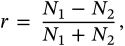
The two-colour fitters (Gaussian 2D 2C, Spline 3D 2C) fit each molecule in both halves at once, with one position and a photon number per half. This plugin turns those two photon numbers into a colour. For every localization it computes the photon split
 and
and  the photons in the two halves.
  runs from
  (all light in the second half) to
  (all in the first). Over a sample with two dyes, the histogram of
  has two peaks, one per dye. The plugin finds them and writes a
 channel column: 1 for the peak at lower  , 2 for the next, and 0 for a localization it will not decide on.
It offers two ways to decide:
 alone, and a fixed band around the boundary is left undecided.
Both fitters run this plugin at the end of every fit (assign colours, in their after the fit section, on by default, with the minima method), so a two-colour table normally arrives with its colours. Run it again from the Analysis tab to see how it decided, or to decide differently.
What it needs. Two columns of photons per localization: photons_ch0 and photons_ch1, as the two-colour fitters write them, or another pair (see channel 1 column). The fit's errors on them, photons_err_ch0 and photons_err_ch1, are used when they are there. The peaks are looked for in the current selection – the layer's filter and the ROI – and the colours are then given to every localization of the table. A filter on channel itself is left out of that selection: after a first run the layers are usually set to one colour each, and the histogram still has to see both dyes. It warns below 50 selected localizations.
1. The split. For every localization the plugin computes  from the two photon numbers, and how precisely that localization measures it. Photons arrive at random, so even a molecule of a known dye does not split its light exactly as the dye does on average: with
  photons in all, the measured
  scatters around the dye's own value
  by
by
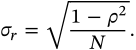
A localization with 1000 photons measures  to about
  ; one with 50 photons only to about
  . This is the whole difference between the two methods: the first ignores it, the second uses it.
2. The peaks. The histogram of  over the selection (histogram bins, 200 over the range
  to
to  ) is smoothed (smoothing, 2 bins), and its highest peaks are the colours (colours, 2). Two peaks closer than three smoothing widths count as one. Each peak's position is refined between the bins. If the ratios of the dyes are known – measured on samples with one dye only, or computed from the spectra – they can be typed in (expected r), and only the boundaries and the share of each colour are then read off the histogram.
3. The boundaries. Between two neighbouring peaks, the boundary is the lowest point of the smoothed histogram. When the valley is flat – two well separated dyes leave a stretch of empty bins – it is the middle of the longest empty stretch. The number of localizations on each side of the boundaries is each colour's share of the sample.
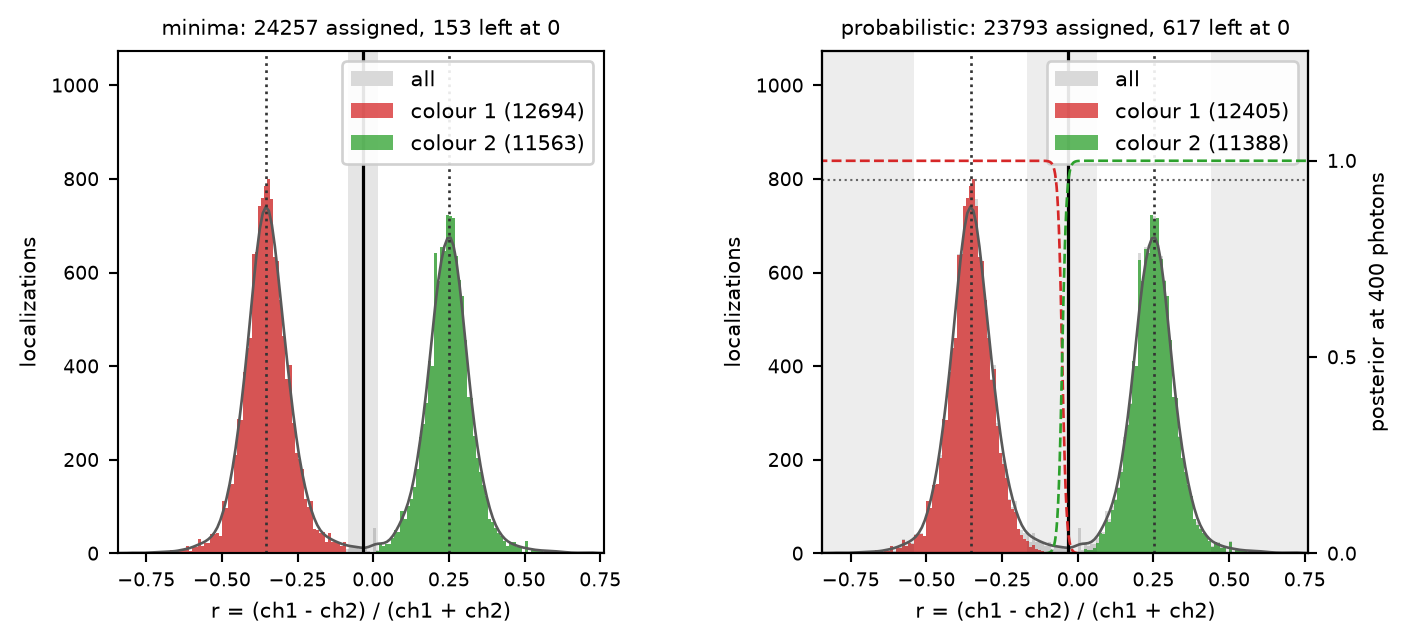
The histogram of  for a simulated sample of two dyes (
 and
and  ), as the plugin draws it. Left: split at the minima. The dotted lines are the peaks, the solid line the boundary, and the grey band around it is left undecided. Right: probabilistic. The dashed curves are the probability of each colour for a localization of median brightness, and the shaded stretches are what such a localization would not be given: the valley between the dyes, and the far tails.
4a. Split at the minima. A localization gets the colour of the side of the boundary it falls on. Within exclusion dr of a boundary it gets 0. The band is the same for every localization, however bright. It has to be wide enough for the dim localizations, whose  is uncertain, and it then throws away bright ones that were perfectly clear.
4b. Probabilistic. Each localization is given the probability of each colour, worked out from its own two photon numbers. The question is: given that the dyes split as the peaks say, how likely is it that this molecule, with these photons on each side, is dye 1 rather than dye 2? How bright the molecule is drops out of the answer; only how its photons divide matters, and how many there are to go by. The answer is weighted by each colour's share of the sample (use abundances).
A colour is then given only if two tests pass:
 ,
,  the allowed crosstalk (5%). Among the localizations that pass, the expected fraction given the wrong colour is then at most
  . This test refuses a narrow band around the boundary, narrow for a bright localization and wide for a dim one.
 must lie within sigma (3) standard deviations of the chosen dye's own ratio, the standard deviation being that localization's own
  plus the extra spread. This test refuses a localization that is neither dye: two molecules of different dyes on at the same place, or a fit that went wrong. The probability cannot do this, because it only compares the colours with each other: a localization exactly between two far-apart peaks still gets a probability near 1 for whichever side it leans to.
5. The intensity plane. The histogram of  divides the brightness out, and the brightness is what the second method depends on. So the plugin draws a second figure (the intensities tab): the photons of one half against those of the other, on log scales. A dye is a straight diagonal line there, because a fixed split is a fixed ratio
  . The coloured regions are where each colour is given; grey is where nothing is.
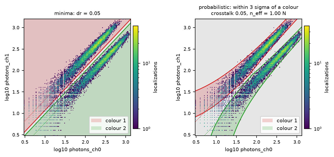
The same localizations in the intensity plane. Left: split at the minima gives each colour a band of fixed width in  , the same for dim and bright molecules. Right: the probabilistic method gives each colour a band that is wide at few photons, where the split is uncertain, and narrow at many, and leaves the space between the dyes grey.
6. How wide the peaks really are. Real peaks are usually wider than the photon statistics alone make them: a dye's split varies between molecules, with its surroundings, or across the field of the splitter. The probabilistic method only knows about the photon statistics unless it is told (extra spread), and without it it refuses bright localizations that sit a little off their dye's ratio. The text therefore compares the strongest peak's measured width with the width the photons explain, and prints the extra spread that would account for the rest.
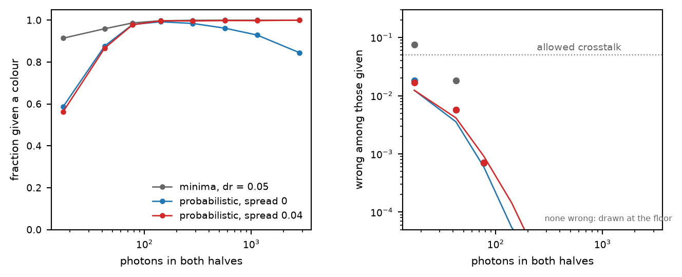
Against the truth, in bins of total photons. Left: the fraction of localizations given a colour. Right: of those, the fraction given the wrong one (points) and, for the probabilistic method, the fraction it expected to get wrong (line). The minima method keeps nearly everything and makes its mistakes among the dim localizations; the probabilistic method refuses the dim ones it cannot tell apart, and with extra spread 0 it also refuses bright localizations whose own split is off their dye's by more than photon noise. The simulated molecules wander by 0.04, which is the spread given to the red curve.
The split and its precision. With  , a localization is used if both counts are finite and
  (and
(and  minimum photons when that is set);
  is clipped to
  , because a fit can put a channel slightly below zero. If each photon of dye
  goes to the first half with probability
  , then
  is binomial and the variance of
  is exactly
  .
.
With the fitted errors  and
and  of the two counts (use fitted errors, and both
 photons_err_* columns present), the variance of  at the measured point is propagated,
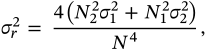
and turned into an effective photon number
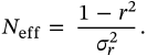
It equals  when the errors are pure shot noise and is smaller when the background under the spot or an EMCCD's excess noise has cost information. Everything below uses
  in place of
  , so the variance keeps its
  form under each dye's hypothesis instead of the plug-in value, which would go to zero at
  and make the most extreme, dimmest localizations look the most certain. Where
  is not a positive finite number – an error missing, or
  exactly
  – the total
  is used. Without error columns,
  throughout.
Finding the peaks. The histogram has histogram bins bins over  and is smoothed with a Gaussian of smoothing bins (0: not smoothed). A bin is a candidate peak if it is non-zero and at least as high as both its neighbours. Candidates are taken highest first, skipping any within
  bins (at least one) of a peak already taken, until there are colours of them; fewer is an error that names the remedies. Each is refined by a parabola through its bin and the two beside it, moved by at most one bin. With expected r, those values are the peaks and nothing is searched.
Boundaries. Between two peaks, the bins at the valley's minimum are found, and the longest contiguous run of them is taken – the one nearest the midpoint of the two peaks if two runs are equally long. The boundary is the middle bin of that run, refined by a parabola. Two peaks less than two bins apart are split halfway. Each colour's share  is the fraction of the selection between the boundaries on either side of it.
The probability of each colour. The two counts of a molecule of dye  with expected brightness
  are independent Poisson numbers, and their joint probability factorises into a Poisson in the total and a binomial in the split,

Only the second factor depends on the dye and only the first on the brightness, so the brightness, whatever its distribution, cancels from the posterior. What is left, evaluated at the effective counts  and
and  , is
, is
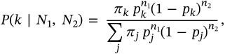
with  for all
  when use abundances is off. For two dyes the log-odds are linear in the counts: every photon adds the same amount of evidence. The binomial is used rather than a Gaussian in
  because the two part company when one half collects few photons – the case of a dye that sends almost all its light to one side.
Extra spread. With extra spread  , a dye's
  is itself drawn from a Beta distribution of mean
  and concentration
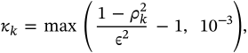
which gives the ratio a standard deviation  in
in  . The split is then beta-binomial – still exact, still independent of the brightness – and the variance of
  under dye
  becomes
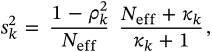
which is shot noise and spread added in quadrature to first order, and exact at both ends. With  ,
,  .
.
The two tests. With  the most probable dye, a localization is given
  if
if

 the allowed crosstalk and
  the sigma tolerance;
  turns the second test off. The first is Chow's rule, a Bayes classifier with a reject option. The chance that an assigned localization is wrong is
  , so requiring
 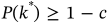 bounds the expected error among the assigned by
  – under the model, which is only as good as the claim that each peak is as wide as its photons and its spread make it. The mean of
  over the assigned localizations is reported as the expected crosstalk, and is usually far below
  , since most localizations are nowhere near a boundary. With keep the tails, the second test is not applied to a localization with
  below the first peak or above the last: there is no other dye out there to be confused with.
How the two methods compare. For two dyes of equal share and the same  , the first test alone refuses a band around the midpoint
  of half-width
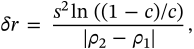
the exclusion zone of the minima method, except that its shot-noise part shrinks as  . The text reports it for the median localization, with
  , as the exclusion dr the minima method would need to match.
Mode width. The strongest peak's width is read off the smoothed histogram: the distance from the peak to where it falls to half its height, interpolated between bins, on each side that crosses half before reaching the neighbouring boundary (both sides averaged when both do). That half-width at half maximum is divided by 1.1774 to give a standard deviation, and the smoothing, in the same units, is taken off in quadrature. It is compared with the median 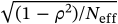 of the localizations on that peak's side of the boundaries,
  ; when the peak's width
  is larger,
  is printed as the extra spread to try.
A population between the peaks. A bump in the smoothed histogram that lies between the first and the last peak, is more than one bin from every chosen peak, and is at least 5% of the height of the lower of the two peaks beside it is named in the text as a warning. It is a population the model does not have – two dyes on in one spot, a third dye – and the minima method hands it whole to one side; the sigma test of the probabilistic method refuses it.
The regions in the intensity plane. The rule depends on the two counts only through  and
and  , so it can be evaluated anywhere. A grid point has no fitted error, so
  there is its total times the table's median
  (shown in the figure's title, kept between 0.001 and 1). Along 260 totals, 2001 values of
  are decided and each colour's first and last are its region's two edges. The view is limited to the 0.1th and 99.9th percentile of each half's photons, the histogram of
  to the 0.1th and 99.9th percentile of
  .
.
Compared with the papers. Reading a molecule's colour from how its photons divide between two detection channels is the method of Bossi et al. 2008. Li et al. 2022 assign colours from a global fit by a threshold on the photon ratio – which is what split at the minima does, with the boundaries found in the histogram rather than set by hand. Li et al. also fit every molecule with the photon ratio fixed at each dye's value and keep the most likely fit; that is not done here. The probabilistic method was worked out for this plugin.
| setting | default | what it does |
|---|---|---|
methodmode | split at the minima | A cut in r, or a posterior per localization. Start with the minima. Switch to probabilistic when the peaks overlap, when the brightness varies a lot, or when a number for the crosstalk is needed. Each method greys out the settings it does not read. Choices: split at the minima; probabilistic |
colourscolors | 2 | How many species the histogram of r holds. More than two works the same way, with a boundary between each pair of neighbouring peaks, up to 6. The peaks are found in the histogram, so every colour needs a visible peak of its own; otherwise give expected r. 1 to 6 |
exclusion drexclusion | 0.05 | Minima: leave this much of r on either side of a boundary unassigned. In units of |
sigmatolerance | 3 | Probabilistic: a colour is given only within this many sigma of its expected split, the sigma being that localization's own photon statistics plus any extra spread. 0: assign to the nearest colour however far away. 3 refuses about 0.3% of the localizations that really are the dye, and anything further out. Much smaller refuses good localizations; 0 gives every localization to its likelier dye, however far away. |
keep the tailskeep_tails | off | Probabilistic: apply the sigma test only between the outermost colours, so a localization more extreme than the first or the last mode is kept rather than refused. Worth turning on when a dye's peak has a long tail on its outer side – a splitter whose ratio changes across the field, say – and those molecules should be kept. |
allowed crosstalkcrosstalk | 0.05 | Probabilistic: refuse what is too close to call as well – the largest expected fraction of wrongly assigned localizations. Narrow beside the sigma test, and what matters where two colours overlap. The band it refuses grows only as |
extra spreadspread | 0 | Probabilistic: a species' own width in r, added in quadrature to the shot noise, for a dye whose splitting ratio varies across the field or between molecules. 0: shot noise alone (the summary prints what the modes suggest). Read it off the text after a first run (colour k is ... wide against ...), and run again. Too small, and bright localizations are refused for being a little off their dye's ratio; too large, and the sigma test lets through what lies between the dyes. |
use fitted errorsuse_errors | on | Take the photon errors from the fit where the table has them; otherwise sqrt(photons). Leave it on. Off, |
use abundances (more)use_prior | on | Probabilistic: weight each species by how much of the sample sits under its mode. Off treats the colours as equally likely beforehand, which gives the rarer colour a little more of the localizations near a boundary. It matters only close to a boundary. |
minimum photons (more)min_photons | 0 | Localizations with fewer photons in total are ignored and left unassigned. The photons of both halves together. |
intensity LUT (more)cmap | viridis | The colour map of the intensity plot's 2D histogram. Only the look of the intensity plot. Choices: viridis; cividis; turbo; magma; inferno; Greys; Greys_r |
histogram bins (more)bins | 200 | How many bins the histogram of r has over its whole range, -1 to 1. Raise it with many localizations and narrow peaks; lower it for a sparse selection, whose histogram is otherwise noisy. 10 to 2000 |
smoothing (more)smoothing | 2 bins | The histogram is smoothed by this much before its maxima are looked for; it also sets how far apart two modes must be. If two dyes are found as one peak, lower it; if one dye is found as two, raise it. |
expected r (more)expected | auto | The species' ratios, comma separated ("-0.65, 0.96"), measured on single-label samples or computed from the spectra. auto: the histogram's own maxima. One value per colour, in any order; they are sorted. Use it when the peaks are not clear in the histogram, or to keep the ratios fixed between samples. |
channel 1 column (more)channel1 | auto | Auto: photons_ch0, or the first pair of per-channel columns in the table. The column |
channel 2 column (more)channel2 | auto | The column r counts negative; name both columns or neither. |
The table gains these columns, for every localization, selected or not, and the run is logged in the file's history:
channel – the colour, 1 for the peak at the lowest  , 2 for the next, and 0 where none was given or the photons are missing.
color_ratio –  .
.channel_p1, channel_p2, ... – the probability of each colour, from the probabilistic model, whichever method decided channel. A probability is only a comparison of the colours with each other: it is near 0 or 1 almost everywhere, also for a localization that is neither.channel_p – the probability of the colour given; 1 for every assigned localization with the minima method, and 0 where channel is 0.channel_sigma – how many standard deviations the nearest dye is from this localization's  . This is the column that tells a localization on a peak from one between the peaks, and a useful filter.
Beside the table:
 (the first figure above), coloured by what was given.
A good result has clear, separate peaks, a boundary in an empty or nearly empty valley, and a strongest peak not much wider than its photon noise (or an extra spread that accounts for the difference). A warning about a population between the peaks, or a boundary on the flank of a peak, means the two colours are not what the histogram holds.
Preview draws both figures and writes the text without changing the table.
Does the job of SMAP's Assign2C/Intensity2Channel (Ries 2020), which draws the two channels' intensities against each other and lets the user type in the lines that divide them (a slope, an offset and an edge excluded on either side). Here:
 , or from expected r.
 . A good value is a little more than
  of the dim localizations (step 1): at 100 photons, about 0.1. 0 decides every localization.
 : going from 5% to 0.1% makes it about 2.4 times as wide. With well separated dyes it hardly matters; it is the sigma test that does most of the refusing.
 : a localization over a high background is then trusted more than it should be.
 counts positive. Name both columns or neither; auto takes the first pair the table has of